Football betting odds can be modeled using the Poisson distribution, a statistical method that predicts how often independent events — like goals in a match — occur over a fixed interval. The approach traces back to 1898, when Russian statistician Ladislaus Bortkiewicz (of Polish ancestry) used it to model Prussian cavalry deaths from horse kicks in his book Das Gesetz der kleinen Zahlen. The distribution itself was formulated by Siméon Denis Poisson in 1837.
Poisson distribution can be used in many scenarios, and one of the most interesting is betting. Sports betting is a global industry valued at approximately $110–$115 billion in 2025, according to market research from Grand View Research and Fortune Business Insights.
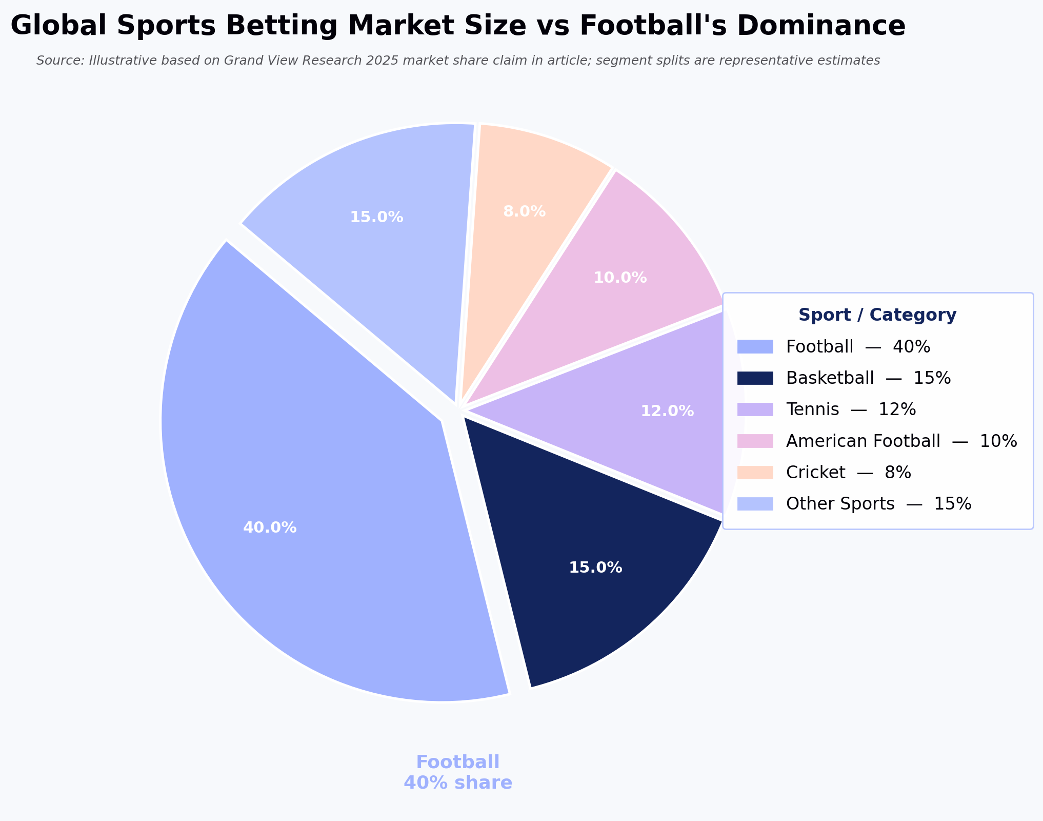
Football is the most-bet-on sport worldwide: according to Grand View Research, football held the largest share of the global sports betting market in 2025.
But how do football betting odds work, and how are they calculated?
What are football betting odds and how do they define bets?

Anyone who has looked at a bookmaker's market has seen the numbers displayed next to each possible outcome.
These numbers are called 'odds' and they define the probabilities of each possible outcome in an event.
The higher the value of these numbers, the less probable that particular event is.
Take the Real Madrid vs Roma match above as an example.
Since the probability of Madrid winning is higher, the odds against them winning is just 1.40. A draw, which is more unlikely, has odds of 4.75.
And the odds of a highly unlikely Roma win in 7.00.
How do these numbers impact your bet amount and their returns?
In the above example, a 1-unit stake on a Real Madrid win at 1.40 returns 1.40 units total, inclusive of the original stake.
Which is why winning bets on more unlikely events (like a Roma victory) gets you bigger returns.
In this case, a winning Roma bet would return 7 units for every 1 unit staked.
What is Poisson distribution?
The Poisson distribution gives the probability of a number of events occurring in a fixed interval, given a known average rate and the assumption that events occur independently of one another.
For instance, suppose you sit in a park for a few days and count the number of people who come to the park in a black T-shirt.
Using Poisson distribution, you can guess if the number of people coming to the park on a specific day in a black t-shirt will be 10, 11, etc.
How does the Poisson distribution relate to football betting odds?
If you are able to calculate the average attack and defense strength of the teams in a match over a certain period and calculate the Poisson distribution, you will be able to predict the odds of one team performing over other.
But if the data is too long the data would be irrelevant, and if it's short, outliers might skew the data.
External factors like transfers and home-vs-away context affect the odds. So does the length of the data window itself, which must be chosen carefully.
Before we apply Poisson, we need to get some mathematical figures.
The following is a pedagogical worked example. The team-level numbers and season totals below are illustrative inputs chosen to demonstrate the mechanics of the Poisson method — they should not be treated as verified 2015–16 EPL statistics or as a real forecast for the 26 February 2017 Manchester derby.
First, we need to find the attack and defense strength of these teams.
Calculating Average Attack and Defense for prediction
Before we identify a particular team strength and weakness, we need to find the average strength and weakness of all teams in the last playing season.
This can be calculated by dividing the total goals scored in particular season by a total number of games played in a particular season.
Using English Premier League 2015–16 season totals (380 matches):
- Number of Goals Scored at Home / Number of Games = 203/380 = 0.534
- Number of Goals Scored Away / Number of Games = 158/380 = 0.415
The difference from the values above gives the "Attack intensity" of a team.
We will also need an average of goals conceded to know the weakness, which is simply the inverse of goals scored.
The average number of goals conceded at Home = 0.415
The average number of goals conceded away = 0.534
This gives us the " Defense intensity" of a team.
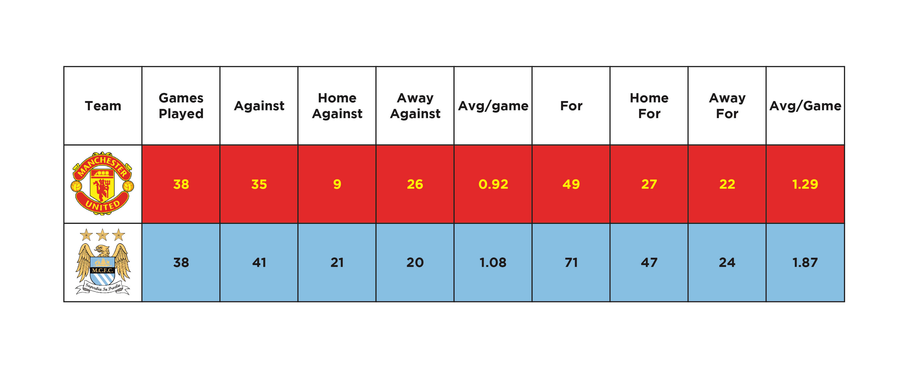
Now that we have the average strength and weakness of the teams, let's take a look at the stats for Manchester United and Manchester City in 2015.
Based on these stats, we can calculate the Poisson distribution for the teams playing in February 2017, where Manchester United is the away team and Manchester City is the home team.
Predicting Manchester United Goals (illustrative figures)
Let's see the possibility of Manchester United scoring at Manchester City's home ground.
Manchester United attack strength (away) = Number of goals scored away / number of away games = 22/19 = 1.15, and dividing by the season's average away goals (0.415) gives an attack-strength multiplier used in the illustrative worked example below.
Manchester City Defense at home
This is calculated by dividing the number of goals conceded at home in the last season by the home team by the number of away games, which is 1.105 ( (21/19).
Manchester City Goals = Number of goals conceded/ Season's average goals conceded = 1.105/0.415 = 2.66
Manchester United's expected goals (λ) = Manchester United's attack strength × Manchester City's defense strength × season's average home goals ≈ 3.05 (illustrative figures)
This expected-goals value (λ) is what feeds directly into the Poisson formula P(x; λ) used to produce the probability table below.
Predicting Manchester City Goals (illustrative figures)
Manchester City Attack at Home
Manchester City = Number of Goals scored home - 47/19 = 2.47
Manchester City Goals = Number of goals scored/Average goals scored in the last season =2.47/0.534 = 4.62
Manchester United Defense away
Take the number of goals conceded away last season by the away team and divide by the number of away games, which is equal to 1.05 ((20/19).
Manchester United Goals = Number of goals conceded/Average goals conceded in the last season =1.05/0.534 =1.966
Manchester City's expected goals (λ) = Manchester City's attack strength × Manchester United's defense strength × season's average away goals ≈ 1.10 (illustrative figures)
This expected-goals value (λ) is what feeds directly into the Poisson formula P(x; λ) used to produce the probability table below.
Once we have the averages of Manchester United's goals and Manchester City's goals, we can use them to calculate the Poisson distribution for a number of goals scored by a particular team . (various goals possibilities).
Poisson distribution betting: predicting multiple football match outcomes
The λ (lambda) values calculated above — the expected number of goals for each team — are the input to the Poisson formula below.
For a refresher on probability and statistical thinking underpinning models like this, see our overview of algorithms and their real-world applications. Readers who want to go deeper into the underlying math may also find our descriptive statistics with Python-NumPy walkthrough useful.
The formula for Poisson distribution is:
P(x; λ) = (e^(-λ)) (λ^x) / x!
e = Euler's constant = 2.718
! = Factorial
x = number of successes of the event
λ = mean (expected) number of events
Below is a minimal C implementation of the Poisson probability mass function. It takes a target number of goals (r) and the expected goals (mean/λ) and returns the probability of exactly r goals occurring.
#include <stdio.h>

#include <math.h>

double factorial(int n) {

  int fact = 1;

  for (int i = 1; i<=n; i++) fact *= i;

  return fact;

}

float poisson(int r, float mean) {

  return (exp((-1) * mean) * pow(mean,r))/factorial(r);

}

int main(int argc, char const *argv[])

{

  printf("%f\n", poisson(1, 1.10));

  return 0;

}
The printf line calls poisson(1, 1.10) — the probability that Manchester City scores exactly 1 goal given their expected goals of 1.10.
If you prefer a spreadsheet, Excel and Google Sheets both provide the POISSON.DIST function. The formula =POISSON.DIST(1, 1.10, FALSE) returns the probability that Manchester City scores exactly 1 goal given expected goals of 1.10. Set the third argument to TRUE for the cumulative probability of 1 or fewer goals.
You can also use the Poisson Distribution Calculator for such equations.
Poisson distribution prediction for the Manchester United vs Manchester City match
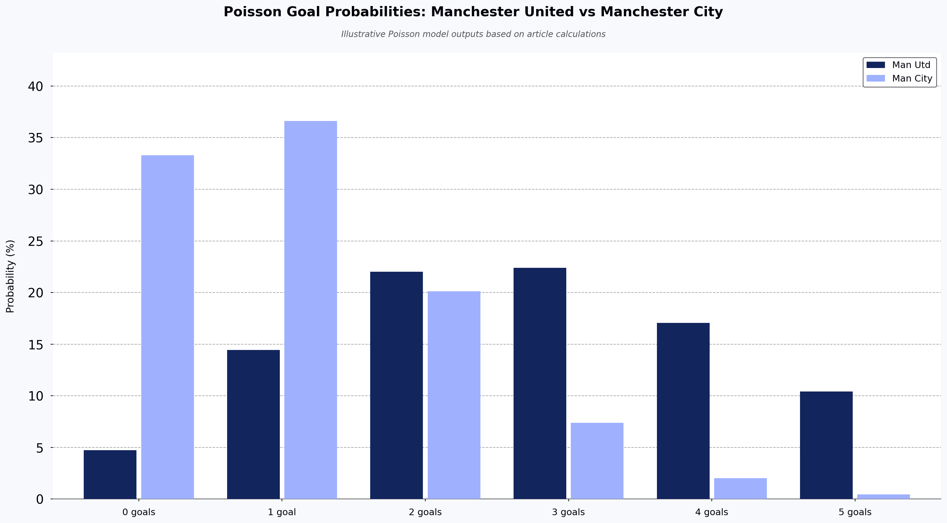
Read this table as a correct-score matrix. The Manchester United and Manchester City rows give each team's individual goal probabilities. The Probability row shows only same-score draws (0-0, 1-1, 2-2, etc.), calculated by multiplying the two team probabilities in that column — for example, the 1-1 draw is 14.44% × 36.61% ≈ 5.28%.
| Goals | 0 | 1 | 2 | 3 | 4 | 5 |
| Manchester United | 4.73% | 14.44% | 22.02% | 22.39% | 17.07% | 10.41% |
| Manchester City | 33.28% | 36.61% | 20.13% | 7.38% | 2.03% | 0.44% |
| Probability | 1.57% | 5.28% | 4.43% | 1.65% | 0.34% | 0.05% |
Read as a correct-score probability matrix, the two team rows let you multiply any Manchester United goal count by any Manchester City goal count to get the probability of that exact scoreline — for example, a 2-1 Manchester City win is 22.02% × 36.61% ≈ 8.06%. To get the full match-outcome probabilities, sum the joint probabilities for every scoreline in each category — all cells where Manchester City goals > Manchester United goals for a City win, all equal-score cells for a draw, and all cells where Manchester United goals > Manchester City goals for a United win.
The possibility that Manchester United and Manchester City would score 1 goal each is 14.44% and 36.61% respectively.
From the distribution table, the probability of Manchester United scoring no goal is 4.73%, and the probability of Manchester City scoring no goal is 33.28%.
Scoring 2 goals, each for Manchester United and Manchester City is 22.02% and 20.13% respectively.
The possibilities decrease as the number of goals increases to 4 and 5 goals by the individual team.
Taking these number into consideration, the odds of Manchester City winning would be high if the number of goals in a match were 0 or 1. But if Manchester United were able to score 2 goals, its probability of winning the match would increase.

Converting Poisson probabilities into betting odds
Once you have the probability of each scoreline, converting to fair decimal odds is a single step: fair odds = 1 / probability. For example, if the model gives a 1-1 draw a 5.28% probability, the fair odds are 1 / 0.0528 ≈ 18.94. Bookmakers then apply an overround — commonly reported in the range of roughly 2–10% depending on the market and operator — to build in their margin, so displayed odds are always shorter than the fair odds. Sum the joint probabilities across all scorelines for each of the three match outcomes: home win, draw, and away win. Comparing those totals to the bookmaker's implied probabilities is how value bets are identified.
How bookmakers turn Poisson probabilities into published odds
Based on the number by distribution table and the probability of these goals in a match, it is clear that a 1-1 draw has the highest possibility of 5.28, followed by 4.43 for a 2-2 draw. But the possibility of Manchester City winning with 1-0 or 2-1 also looks great.
Based on the previous match at Old Trafford, which is the home ground to Manchester United, Manchester City won by 2-1.
Based purely on the model, the highest-probability outcomes are a 1-1 draw or a 1-0 Manchester City win.
The main limitation of the standard Poisson model is that it ignores external factors like transfers, coaching changes, injuries, and home-ground effects, and it treats goals as fully independent events — which understates the frequency of low-scoring draws such as 0-0 and 1-1. The Dixon-Coles (1997) adjustment is the standard academic correction, re-weighting low-scoring outcomes to better match observed match data. More sophisticated models also add recency weighting and model home advantage explicitly rather than folding it into raw averages.
FAQ: football betting odds and Poisson distribution
Q: When should you use a Poisson distribution in football betting?
A: Poisson applies generally when you are modeling counts of independent events that occur at a roughly constant average rate over a fixed interval. In football, that maps to modeling the number of goals each team scores in 90 minutes, provided goals are treated as independent events.
Q: Can Poisson distribution accurately predict football scores?
A: It gives a reasonable baseline for score probabilities but understates low-scoring draws (0-0, 1-1) and ignores factors like injuries, transfers, and home advantage. The Dixon-Coles adjustment is often used to correct for these effects.
Q: How do you convert Poisson probabilities into betting odds?
A: Take the reciprocal of the modeled probability, then compare that fair price to the bookmaker's displayed odds — if the bookmaker's implied probability is lower than yours, the bet has positive expected value. That comparison, not the reciprocal itself, is where edge is found.
Q: What is the most profitable betting strategy when using a Poisson model?
A: There is no single most profitable strategy — profitability comes from three disciplines working together. First, calibrate the model on a rolling window (typically 20-40 recent matches per team) to avoid stale or noisy inputs. Second, only place bets when your fair-odds edge exceeds the bookmaker overround plus a safety buffer of around 2%. Third, use fractional Kelly staking (commonly one-quarter to one-half Kelly) to size bets in proportion to edge while limiting variance.
Q: What is the 80/20 rule in sports betting?
A: The 80/20 rule is a general heuristic sometimes cited in betting communities — the idea that a small share of bets or markets produces most of the profit. It is not a formal statistical concept and is unrelated to the Poisson model discussed here, which is a probability distribution for modeling goal counts.
Next steps
Build and validate your own probabilistic models against real match data. Explore HackerEarth's algorithm challenges to practice the statistical and coding techniques used in models like Dixon-Coles and bivariate Poisson.