Introduction
Last week, we learned about Random Forest Algorithm. Now we know it helps us reduce a model's variance by building models on resampled data and thereby increases its generalization capability. Good!
Now, you might be wondering, what to do next for increasing a model's prediction accuracy ? After all, an ideal model is one which is good at both generalization and prediction accuracy. This brings us to Boosting Algorithms.
Developed in 1989, the family of boosting algorithms has been improved over the years. In this article, we'll learn about XGBoost algorithm.
XGBoost is the most popular machine learning algorithm these days. Regardless of the data type (regression or classification), it is well known to provide better solutions than other ML algorithms. In fact, since its inception (early 2014), it has become the "true love" of kaggle users to deal with structured data. So, if you are planning to compete on Kaggle, xgboost is one algorithm you need to master.
In this article, you'll learn about core concepts of the XGBoost algorithm. In addition, we'll look into its practical side, i.e., improving the xgboost model using parameter tuning in R.
On 5th March 2017: How to win Machine Learning Competitions ?
Table of Contents
- What is XGBoost? Why is it so good?
- How does XGBoost work?
- Understanding XGBoost Tuning Parameters
- Practical - Tuning XGBoost using R

What is XGBoost ? Why is it so good ?
XGBoost (Extreme Gradient Boosting) is an optimized distributed gradient boosting library. Yes, it uses gradient boosting (GBM) framework at core. Yet, does better than GBM framework alone. XGBoost was created by Tianqi Chen, PhD Student, University of Washington. It is used for supervised ML problems. Let's look at what makes it so good:
- Parallel Computing: It is enabled with parallel processing (using OpenMP); i.e., when you run xgboost, by default, it would use all the cores of your laptop/machine.
- Regularization: I believe this is the biggest advantage of xgboost. GBM has no provision for regularization. Regularization is a technique used to avoid overfitting in linear and tree-based models.
- Enabled Cross Validation: In R, we usually use external packages such as caret and mlr to obtain CV results. But, xgboost is enabled with internal CV function (we'll see below).
- Missing Values: XGBoost is designed to handle missing values internally. The missing values are treated in such a manner that if there exists any trend in missing values, it is captured by the model.
- Flexibility: In addition to regression, classification, and ranking problems, it supports user-defined objective functions also. An objective function is used to measure the performance of the model given a certain set of parameters. Furthermore, it supports user defined evaluation metrics as well.
- Availability: Currently, it is available for programming languages such as R, Python, Java, Julia, and Scala.
- Save and Reload: XGBoost gives us a feature to save our data matrix and model and reload it later. Suppose, we have a large data set, we can simply save the model and use it in future instead of wasting time redoing the computation.
- Tree Pruning: Unlike GBM, where tree pruning stops once a negative loss is encountered, XGBoost grows the tree upto max_depth and then prune backward until the improvement in loss function is below a threshold.
I'm sure now you are excited to master this algorithm. But remember, with great power comes great difficulties too. You might learn to use this algorithm in a few minutes, but optimizing it is a challenge. Don't worry, we shall look into it in following sections.
How does XGBoost work ?
XGBoost belongs to a family of boosting algorithms that convert weak learners into strong learners. A weak learner is one which is slightly better than random guessing. Let's understand boosting first (in general).
Boosting is a sequential process; i.e., trees are grown using the information from a previously grown tree one after the other. This process slowly learns from data and tries to improve its prediction in subsequent iterations. Let's look at a classic classification example:
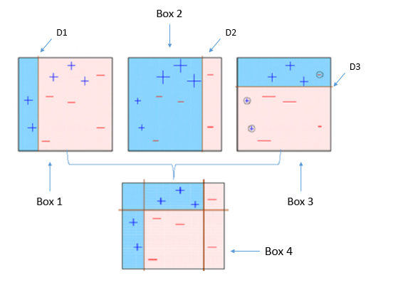
Four classifiers (in 4 boxes), shown above, are trying hard to classify + and - classes as homogeneously as possible. Let's understand this picture well.
- Box 1: The first classifier creates a vertical line (split) at D1. It says anything to the left of D1 is
+ and anything to the right of D1 is -. However, this classifier misclassifies three + points.
- Box 2: The next classifier says don't worry I will correct your mistakes. Therefore, it gives more weight to the three
+ misclassified points (see bigger size of +) and creates a vertical line at D2. Again it says, anything to right of D2 is - and left is +. Still, it makes mistakes by incorrectly classifying three - points.
- Box 3: The next classifier continues to bestow support. Again, it gives more weight to the three
- misclassified points and creates a horizontal line at D3. Still, this classifier fails to classify the points (in circle) correctly.
- Remember that each of these classifiers has a misclassification error associated with them.
- Boxes 1,2, and 3 are weak classifiers. These classifiers will now be used to create a strong classifier Box 4.
- Box 4: It is a weighted combination of the weak classifiers. As you can see, it does good job at classifying all the points correctly.
That's the basic idea behind boosting algorithms. The very next model capitalizes on the misclassification/error of previous model and tries to reduce it. Now, let's come to XGBoost.
As we know, XGBoost can used to solve both regression and classification problems. It is enabled with separate methods to solve respective problems. Let's see:
Classification Problems: To solve such problems, it uses booster = gbtree parameter; i.e., a tree is grown one after other and attempts to reduce misclassification rate in subsequent iterations. In this, the next tree is built by giving a higher weight to misclassified points by the previous tree (as explained above).
Regression Problems: To solve such problems, we have two methods: booster = gbtree and booster = gblinear. You already know gbtree. In gblinear, it builds generalized linear model and optimizes it using regularization (L1,L2) and gradient descent. In this, the subsequent models are built on residuals (actual - predicted) generated by previous iterations. Are you wondering what is gradient descent? Understanding gradient descent requires math, however, let me try and explain it in simple words:
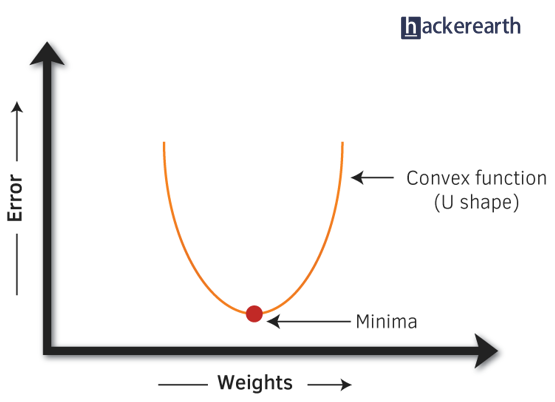
- Gradient Descent: It is a method which comprises a vector of weights (or coefficients) where we calculate their partial derivative with respective to zero. The motive behind calculating their partial derivative is to find the local minima of the loss function (RSS), which is convex in nature. In simple words, gradient descent tries to optimize the loss function by tuning different values of coefficients to minimize the error.
Hopefully, up till now, you have developed a basic intuition around how boosting and xgboost works. Let's proceed to understand its parameters. After all, using xgboost without parameter tuning is like driving a car without changing its gears; you can never up your speed.
Note: In R, xgboost package uses a matrix of input data instead of a data frame.
Understanding XGBoost Tuning Parameters
Every parameter has a significant role to play in the model's performance. Before hypertuning, let's first understand about these parameters and their importance. In this article, I've only explained the most frequently used and tunable parameters. To look at all the parameters, you can refer to its official documentation.
XGBoost parameters can be divided into three categories (as suggested by its authors):
- General Parameters: Controls the booster type in the model which eventually drives overall functioning
- Booster Parameters: Controls the performance of the selected booster
- Learning Task Parameters: Sets and evaluates the learning process of the booster from the given data
- General Parameters
- Booster[default=gbtree]
- Sets the booster type (gbtree, gblinear or dart) to use. For classification problems, you can use gbtree, dart. For regression, you can use any.
- nthread[default=maximum cores available]
- Activates parallel computation. Generally, people don't change it as using maximum cores leads to the fastest computation.
- silent[default=0]
- If you set it to 1, your R console will get flooded with running messages. Better not to change it.
- Booster Parameters
As mentioned above, parameters for tree and linear boosters are different. Let's understand each one of them:
Parameters for Tree Booster
- nrounds[default=100]
- It controls the maximum number of iterations. For classification, it is similar to the number of trees to grow.
- Should be tuned using CV
- eta[default=0.3][range: (0,1)]
- It controls the learning rate, i.e., the rate at which our model learns patterns in data. After every round, it shrinks the feature weights to reach the best optimum.
- Lower eta leads to slower computation. It must be supported by increase in
nrounds.
- Typically, it lies between 0.01 - 0.3
- gamma[default=0][range: (0,Inf)]
- It controls regularization (or prevents overfitting). The optimal value of gamma depends on the data set and other parameter values.
- Higher the value, higher the regularization. Regularization means penalizing large coefficients which don't improve the model's performance.
default = 0 means no regularization.
- Tune trick: Start with 0 and check CV error rate. If you see train error >>> test error, bring gamma into action. Higher the gamma, lower the difference in train and test CV. If you have no clue what value to use, use gamma=5 and see the performance. Remember that gamma brings improvement when you want to use shallow (low
max_depth) trees.
- max_depth[default=6][range: (0,Inf)]
- It controls the depth of the tree.
- Larger the depth, more complex the model; higher chances of overfitting. There is no standard value for max_depth. Larger data sets require deep trees to learn the rules from data.
- Should be tuned using CV
- min_child_weight[default=1][range:(0,Inf)]
- In regression, it refers to the minimum number of instances required in a child node. In classification, if the leaf node has a minimum sum of instance weight (calculated by second order partial derivative) lower than min_child_weight, the tree splitting stops.
- In simple words, it blocks the potential feature interactions to prevent overfitting. Should be tuned using CV.
- subsample[default=1][range: (0,1)]
- It controls the number of samples (observations) supplied to a tree.
- Typically, its values lie between (0.5-0.8)
- colsample_bytree[default=1][range: (0,1)]
- It control the number of features (variables) supplied to a tree
- Typically, its values lie between (0.5,0.9)
- lambda[default=0]
- It controls L2 regularization (equivalent to Ridge regression) on weights. It is used to avoid overfitting.
- alpha[default=1]
- It controls L1 regularization (equivalent to Lasso regression) on weights. In addition to shrinkage, enabling alpha also results in feature selection. Hence, it's more useful on high dimensional data sets.
Parameters for Linear Booster
Using linear booster has relatively lesser parameters to tune, hence it computes much faster than gbtree booster.
- nrounds[default=100]
- It controls the maximum number of iterations (steps) required for gradient descent to converge.
- Should be tuned using CV
- lambda[default=0]
- It enables Ridge Regression. Same as above
- alpha[default=1]
- It enables Lasso Regression. Same as above
- Learning Task Parameters
These parameters specify methods for the loss function and model evaluation. In addition to the parameters listed below, you are free to use a customized objective / evaluation function.
- Objective[default=reg:linear]
- reg:linear - for linear regression
- binary:logistic - logistic regression for binary classification. It returns class probabilities
- multi:softmax - multiclassification using softmax objective. It returns predicted class labels. It requires setting
num_class parameter denoting number of unique prediction classes.
- multi:softprob - multiclassification using softmax objective. It returns predicted class probabilities.
- eval_metric [no default, depends on objective selected]
- These metrics are used to evaluate a model's accuracy on validation data. For regression, default metric is
RMSE. For classification, default metric is error.
- Available error functions are as follows:
- mae - Mean Absolute Error (used in regression)
- Logloss - Negative loglikelihood (used in classification)
- AUC - Area under curve (used in classification)
- RMSE - Root mean square error (used in regression)
- error - Binary classification error rate [#wrong cases/#all cases]
- mlogloss - multiclass logloss (used in classification)
We've looked at how xgboost works, the significance of each of its tuning parameter, and how it affects the model's performance. Let's bolster our newly acquired knowledge by solving a practical problem in R.
Practical - Tuning XGBoost in R
In this practical section, we'll learn to tune xgboost in two ways: using the xgboost package and MLR package. I don't see the xgboost R package having any inbuilt feature for doing grid/random search. To overcome this bottleneck, we'll use MLR to perform the extensive parametric search and try to obtain optimal accuracy.
I'll use the adult data set from my previous random forest tutorial. This data set poses a classification problem where our job is to predict if the given user will have a salary <=50K or >50K.
Using random forest, we achieved an accuracy of 85.8%. Theoretically, xgboost should be able to surpass random forest's accuracy. Let's see if we can do it. I'll follow the most common but effective steps in parameter tuning:
- First, you build the xgboost model using default parameters. You might be surprised to see that default parameters sometimes give impressive accuracy.
- If you get a depressing model accuracy, do this: fix
eta = 0.1, leave the rest of the parameters at default value, using xgb.cv function get best n_rounds. Now, build a model with these parameters and check the accuracy.
- Otherwise, you can perform a grid search on rest of the parameters (
max_depth, gamma, subsample, colsample_bytree etc) by fixing eta and nrounds. Note: If using gbtree, don't introduce gamma until you see a significant difference in your train and test error.
- Using the best parameters from grid search, tune the regularization parameters(alpha,lambda) if required.
- At last, increase/decrease eta and follow the procedure. But remember, excessively lower
eta values would allow the model to learn deep interactions in the data and in this process, it might capture noise. So be careful!
This process might sound a bit complicated, but it's quite easy to code in R. Don't worry, I've demonstrated all the steps below. Let's get into actions now and quickly prepare our data for modeling (if you don't understand any line of code, ask me in comments):
# set working directory
path <- "~/December 2016/XGBoost_Tutorial"
setwd(path)

# load libraries
library(data.table)
library(mlr)

# set variable names
setcol <- c("age",
            "workclass",
            "fnlwgt",
            "education",
            "education-num",
            "marital-status",
            "occupation",
            "relationship",
            "race",
            "sex",
            "capital-gain",
            "capital-loss",
            "hours-per-week",
            "native-country",
            "target")

# load data
train <- read.table("adultdata.txt", header = FALSE, sep = ",",
                    col.names = setcol, na.strings = c(" ?"),
                    stringsAsFactors = FALSE)
test <- read.table("adulttest.txt", header = FALSE, sep = ",",
                   col.names = setcol, skip = 1,
                   na.strings = c(" ?"), stringsAsFactors = FALSE)

# convert data frame to data table
setDT(train)
setDT(test)

# check missing values
table(is.na(train))
sapply(train, function(x) sum(is.na(x)) / length(x)) * 100
table(is.na(test))
sapply(test, function(x) sum(is.na(x)) / length(x)) * 100

# quick data cleaning
# remove extra character from target variable
library(stringr)
test[, target := substr(target, start = 1, stop = nchar(target) - 1)]

# remove leading whitespaces
char_col <- colnames(train)[sapply(test, is.character)]
for (i in char_col) set(train, j = i, value = str_trim(train[[i]], side = "left"))
for (i in char_col) set(test, j = i, value = str_trim(test[[i]], side = "left"))

# set all missing value as "Missing"
train[is.na(train)] <- "Missing"
test[is.na(test)] <- "Missing"
Up to this point, we dealt with basic data cleaning and data inconsistencies. To use xgboost package, keep these things in mind:
- Convert the categorical variables into numeric using one hot encoding
- For classification, if the dependent variable belongs to class factor, convert it to numeric
R's base function model.matrix is quick enough to implement one hot encoding. In the code below, ~.+0 leads to encoding of all categorical variables without producing an intercept. Alternatively, you can use the dummies package to accomplish the same task. Since xgboost package accepts target variable separately, we'll do the encoding keeping this in mind:
# using one hot encoding
>labels <- train$target
>ts_label <- test$target
>new_tr <- model.matrix(~.+0, data = train[,-c("target"), with = FALSE])
>new_ts <- model.matrix(~.+0, data = test[,-c("target"), with = FALSE])

# convert factor to numeric
>labels <- as.numeric(labels) - 1
>ts_label <- as.numeric(ts_label) - 1
For xgboost, we'll use xgb.DMatrix to convert data table into a matrix (most recommended):
# preparing matrix
>dtrain <- xgb.DMatrix(data = new_tr, label = labels)
&t;dtest <- xgb.DMatrix(data = new_ts, label = ts_label)
As mentioned above, we'll first build our model using default parameters, keeping random forest's accuracy 85.8% in mind. I'll capture the default parameters from above (written against every parameter):
# default parameters
params <- list(
    booster = "gbtree",
    objective = "binary:logistic",
    eta = 0.3,
    gamma = 0,
    max_depth = 6,
    min_child_weight = 1,
    subsample = 1,
    colsample_bytree = 1
)
Using the inbuilt xgb.cv function, let's calculate the best nround for this model. In addition, this function also returns CV error, which is an estimate of test error.
xgbcv <- xgb.cv(
    params = params,
    data = dtrain,
    nrounds = 100,
    nfold = 5,
    showsd = TRUE,
    stratified = TRUE,
    print.every.n = 10,
    early.stop.round = 20,
    maximize = FALSE
)
# best iteration = 79
The model returned lowest error at the 79th (nround) iteration. Also, if you noticed the running messages in your console, you would have understood that train and test error are following each other. We'll use this insight in the following code. Now, we'll see our CV error:
min(xgbcv$test.error.mean)
# 0.1263
As compared to my previous random forest model, this CV accuracy (100-12.63)=87.37% looks better already. However, I believe cross-validation accuracy is usually more optimistic than true test accuracy. Let's calculate our test set accuracy and determine if this default model makes sense:
# first default - model training
xgb1 <- xgb.train(
    params = params,
    data = dtrain,
    nrounds = 79,
    watchlist = list(val = dtest, train = dtrain),
    print.every.n = 10,
    early.stop.round = 10,
    maximize = FALSE,
    eval_metric = "error"
)

# model prediction
xgbpred <- predict(xgb1, dtest)
xgbpred <- ifelse(xgbpred > 0.5, 1, 0)
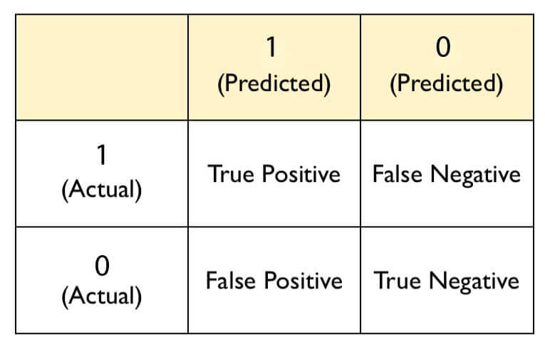
The objective function binary:logistic returns output predictions rather than labels. To convert it, we need to manually use a cutoff value. As seen above, I've used 0.5 as my cutoff value for predictions. We can calculate our model's accuracy using confusionMatrix() function from caret package.
# confusion matrix
library(caret)
confusionMatrix(xgbpred, ts_label)
# Accuracy - 86.54%

# view variable importance plot
mat <- xgb.importance(feature_names = colnames(new_tr), model = xgb1)
xgb.plot.importance(importance_matrix = mat[1:20])  # first 20 variables

As you can see, we've achieved better accuracy than a random forest model using default parameters in xgboost. Can we still improve it? Let's proceed to the random / grid search procedure and attempt to find better accuracy. From here on, we'll be using the MLR package for model building. A quick reminder, the MLR package creates its own frame of data, learner as shown below. Also, keep in mind that task functions in mlr doesn't accept character variables. Hence, we need to convert them to factors before creating task:
# convert characters to factors
fact_col <- colnames(train)[sapply(train, is.character)]
for (i in fact_col) set(train, j = i, value = factor(train[[i]]))
for (i in fact_col) set(test, j = i, value = factor(test[[i]]))

# create tasks
traintask <- makeClassifTask(data = train, target = "target")
testtask <- makeClassifTask(data = test, target = "target")

# do one hot encoding
traintask <- createDummyFeatures(obj = traintask, target = "target")
testtask <- createDummyFeatures(obj = testtask, target = "target")
Now, we'll set the learner and fix the number of rounds and eta as discussed above.
#create learner
# create learner
lrn <- makeLearner("classif.xgboost", predict.type = "response")
lrn$par.vals <- list(
    objective = "binary:logistic",
    eval_metric = "error",
    nrounds = 100L,
    eta = 0.1
)

# set parameter space
params <- makeParamSet(
    makeDiscreteParam("booster", values = c("gbtree", "gblinear")),
    makeIntegerParam("max_depth", lower = 3L, upper = 10L),
    makeNumericParam("min_child_weight", lower = 1L, upper = 10L),
    makeNumericParam("subsample", lower = 0.5, upper = 1),
    makeNumericParam("colsample_bytree", lower = 0.5, upper = 1)
)

# set resampling strategy
rdesc <- makeResampleDesc("CV", stratify = TRUE, iters = 5L)
With stratify=T, we'll ensure that distribution of target class is maintained in the resampled data sets. If you've noticed above, in the parameter set, I didn't consider gamma for tuning. Simply because during cross validation, we saw that train and test error are in sync with each other. Had either one of them been dragging or rushing, we could have brought this parameter into action.
Now, we'll set the search optimization strategy. Though, xgboost is fast, instead of grid search, we'll use random search to find the best parameters.