Manish Saraswat

Author
Manish Saraswat

Blogs
Manish sees hiring through the lens of systems thinking and design operations. Their structured yet poetic approach to writing helps readers rethink how they scale teams and workflows.
author’s Articles

Insights & Stories by Manish Saraswat

From hiring pipelines to collaboration rituals, Manish Saraswat maps out ways to design intentional, high-performing organizations—one post at a time.
Clear all
Thank you! Your submission has been received!
Oops! Something went wrong while submitting the form.
Filter
Filter

Feature Engineering + H2o Gradient Boosting (GBM) in R Scores 0.936

With less than 3 days to go, this script is meant to help beginners with feisty ideas, machine learning workflow and motivation for ongoing machine learning challenge.Here's a quick workflow of what I've done below:
  1. Load data and explore
  2. Data Pre-processing
  3. Dropped Features
  4. One Hot Encoding
  5. Feature Engineering
  6. Model Training
Good Luck!Note: For more feature engineering ideas, spend time on exploring data by loan_status variable. For categorical vs categorical data, create dodged bar plots. For categorical vs continuous data, create density plots and use fill=as.factor(loan_status).

To help the community, feel free to contribute the equivalent python / C ++ script in the comments below.

Update: You can get python script for this solution from Jin Cong Ho's comment below.

Script (R)

Resources - Handy Algorithms for this Challenge

Practical Guide to Clustering Algorithms and Evaluation in R

Introduction

Clustering algorithms are a part of unsupervised machine learning algorithms. As there is no target variable, the model is trained using input variables to discover intrinsic groups or clusters.

Because we don’t have labels for the data, these groups are formed based on similarity between data points. This tutorial covers clustering concepts, techniques, and applications across domains like healthcare, retail, and manufacturing.

We’ll also walk through examples in R, using real-world data from a water treatment plant to apply our knowledge practically.

Table of Contents

  1. Types of Clustering Techniques
  2. Distance Calculation for Clustering
  3. K-Means Clustering
  4. Choosing the Best K in K-Means
  5. Hierarchical Clustering
  6. Evaluation Methods in Cluster Analysis
  7. Clustering in R – Water Treatment Plants

Types of Clustering Techniques

Common clustering algorithms include K-Means, Fuzzy C-Means, and Hierarchical Clustering. Depending on the data type (numeric, categorical, mixed), the algorithm may vary. Clustering techniques can be classified as:

  • Soft Clustering – Observations are assigned to clusters with probabilities.
  • Hard Clustering – Observations belong to only one cluster.

We’ll focus on K-Means and Hierarchical Clustering in this guide.

Distance Calculation for Clustering

Distance metrics are used to measure similarity between data points. Common metrics include:

  • Euclidean Distance – Suitable for numeric variables.
  • Manhattan Distance – Measures horizontal and vertical distances.
  • Hamming Distance – Used for categorical variables.
  • Gower Distance – Handles mixed variable types.
  • Cosine Similarity – Common in text analysis.

K-Means Clustering

K-Means partitions data into k non-overlapping clusters. The process includes:

  1. Randomly assign k centroids.
  2. Assign observations to the nearest centroid.
  3. Recalculate centroids.
  4. Repeat until convergence.

Clustering minimizes within-cluster variation using squared Euclidean distance.

Choosing the Best K in K-Means

Methods for selecting k include:

  • Cross Validation
  • Elbow Method
  • Silhouette Method
  • X-Means Clustering

Hierarchical Clustering

This method creates a nested sequence of clusters using two approaches:

  • Agglomerative – Bottom-up merging.
  • Divisive – Top-down splitting.

Dendrograms visualize the clustering hierarchy. A horizontal cut across the dendrogram reveals the number of clusters.

Evaluation Methods

Clustering evaluation is divided into:

  • Internal Measures – Based on compactness and separation (e.g., SSE, Scatter Criteria).
  • External Measures – Based on known labels (e.g., Rand Index, Precision-Recall).

Clustering in R – Water Treatment Plants

The water treatment dataset from the UCI repository is used to demonstrate hierarchical and k-means clustering.

# Load and preprocess data
library(data.table)
library(ggplot2)
library(fpc)

water_data <- read.table("water-treatment.data.txt", sep = ",", header = F, na.strings = "?")
setDT(water_data)

# Impute missing values
for(i in colnames(water_data)[-1]) {
  set(water_data, which(is.na(water_data[[i]])), i, median(water_data[[i]], na.rm = TRUE))
}

# Scale numeric features
scaled_wd <- scale(water_data[,-1, with = FALSE])

Next, hierarchical clustering is performed using Euclidean distance and Ward's method. A dendrogram is plotted, and clusters are determined via horizontal cuts. PCA is used to visualize clusters.

# Hierarchical clustering
d <- dist(scaled_wd, method = "euclidean")
h_clust <- hclust(d, method = "ward.D2")
plot(h_clust, labels = water_data$V1)

# Cut dendrogram
rect.hclust(h_clust, k = 4)
groups <- cutree(h_clust, k = 4)

Principal components are used for cluster visualization:

# PCA for visualization
pcmp <- princomp(scaled_wd)
pred_pc <- predict(pcmp)[,1:2]
comp_dt <- cbind(as.data.table(pred_pc), cluster = as.factor(groups), Labels = water_data$V1)

ggplot(comp_dt, aes(Comp.1, Comp.2)) +
  geom_point(aes(color = cluster), size = 3)

Then, k-means clustering is applied and similarly visualized using PCA components. The clustering consistency is confirmed visually.

# K-means clustering
kclust <- kmeans(scaled_wd, centers = 4, iter.max = 100)

ggplot(comp_dt, aes(Comp.1, Comp.2)) +
  geom_point(aes(color = as.factor(kclust$cluster)), size = 3)

How can R Users Learn Python for Data Science ?

Introduction

The best way to learn a new skill is by doing it!

This article is meant to help R users enhance their set of skills and learn Python for data science (from scratch). After all, R and Python are the most important programming languages a data scientist must know.

Python is a supremely powerful and a multi-purpose programming language. It has grown phenomenally in the last few years. It is used for web development, game development, and now data analysis / machine learning. Data analysis and machine learning is a relatively new branch in python.

For a beginner in data science, learning python for data analysis can be really painful. Why?

You try Googling "learn python," and you'll get tons of tutorials only meant for learning python for web development. How can you find a way then?

In this tutorial, we'll be exploring the basics of python for performing data manipulation tasks. Alongside, we'll also look how you do it in R. This parallel comparison will help you relate the set of tasks you do in R to how you do it in python! And in the end, we'll take up a data set and practice our newly acquired python skills.

Note: This article is best suited for people who have a basic knowledge of R language.

Machine learning challenge, ML challenge

Table of Contents

  1. Why learn Python (even if you already know R)
  2. Understanding Data Types and Structures in Python vs. R
  3. Writing Code in Python vs. R
  4. Practicing Python on a Data Set

Why learn Python (even if you already know R)

No doubt, R is tremendously great at what it does. In fact, it was originally designed for doing statistical computing and manipulations. Its incredible community support allows a beginner to learn R quickly.

But, python is catching up fast. Established companies and startups have embraced python at a much larger scale compared to R.

r machine learning vs python machine learning

According to indeed.com (from Jan 2016 to November 2016), the number of job postings seeking "machine learning python" increased much faster (approx. 123%) than "machine learning in R" jobs. Do you know why? It is because

  1. Python supports the entire spectrum of machine learning in a much better way.
  2. Python not only supports model building but also supports model deployment.
  3. The support of various powerful deep learning libraries such as keras, convnet, theano, and tensorflow is more for python than R.
  4. You don't need to juggle between several packages to locate a function in python unlike you do in R. Python has relatively fewer libraries, with each having all the functions a data scientist would need.

Understanding Data Types and Structures in Python vs. R

These programming languages understand the complexity of a data set based on its variables and data types. Yes! Let's say you have a data set with one million rows and 50 columns. How would these programming languages understand the data?

Basically, both R and Python have pre-defined data types. The dependent and independent variables get classified among these data types. And, based on the data type, the interpreter allots memory for use. Python supports the following data types:

  1. Numbers – It stores numeric values. These numeric values can be stored in 4 types: integer, long, float, and complex.
    • Integer – Whole numbers such as 10, 13, 91, 102. Same as R's integer type.
    • Long – Long integers in octa and hexadecimal. R uses bit64 package for hexadecimal.
    • Float – Decimal values like 1.23, 9.89. Equivalent to R's numeric type.
    • Complex – Numbers like 2 + 3i, 5i. Rarely used in data analysis.
  2. Boolean – Stores two values (True and False). R uses factor or character. Case-sensitive difference exists: R uses TRUE/FALSE; Python uses True/False.
  3. Strings – Stores text like "elephant", "lotus". Same as R's character type.
  4. Lists – Like R’s list, stores multiple data types in one structure.
  5. Tuples – Similar to immutable vectors in R (though R has no direct equivalent).
  6. Dictionary – Key-value pair structure. Think of keys as column names, values as data entries.

Since R is a statistical computing language, all the functions to manipulate data and reading variables are available inherently. On the other hand, python hails all the data analysis / manipulation / visualization functions from external libraries. Python has several libraries for data manipulation and machine learning. The most important ones are:

  1. Numpy – Used for numerical computing. Offers math functions and array support. Similar to R’s list or array.
  2. Scipy – Scientific computing in python.
  3. Matplotlib – For data visualization. R uses ggplot2.
  4. Pandas – Main tool for data manipulation. R uses dplyr, data.table.
  5. Scikit Learn – Core library for machine learning algorithms in python.

In a way, python for a data scientist is largely about mastering the libraries stated above. However, there are many more advanced libraries which people have started using. Therefore, for practical purposes you should remember the following things:

  1. Array – Similar to R's list, supports multidimensional data with coercion effect when data types differ.
  2. List – Equivalent to R’s list.
  3. Data Frame – Two-dimensional structure composed of lists. R uses data.frame; python uses DataFrame from pandas.
  4. Matrix – Multidimensional structure of same class data. In R: matrix(); in python: numpy.column_stack().

Until here, I hope you've understood the basics of data types and data structures in R and Python. Now, let's start working with them!

Writing Code in Python vs. R

Let's use the knowledge gained in the previous section and understand its practical implications. But before that, you should install python using Anaconda's Jupyter Notebook. You can download here. Also, you can download other python IDEs. I hope you already have R Studio installed.

1. Creating Lists

In R:

my_list <- list('monday','specter',24,TRUE)
typeof(my_list)
[1] "list"

In Python:

my_list = ['monday','specter',24,True]
type(my_list)
list

Using pandas Series:

import pandas as pd
pd_list = pd.Series(my_list)
pd_list
0     monday
1    specter
2         24
3       True
dtype: object

Python uses zero-based indexing; R uses one-based indexing.

2. Matrix

In R:

my_mat <- matrix(1:10, nrow = 5)
my_mat
     [,1] [,2]
[1,]    1    6
[2,]    2    7
[3,]    3    8
[4,]    4    9
[5,]    5   10

# Select first row
my_mat[1,]

# Select second column
my_mat[,2]

In Python (using NumPy):

import numpy as np
a = np.array(range(10,15))
b = np.array(range(20,25))
c = np.array(range(30,35))
my_mat = np.column_stack([a, b, c])

# Select first row
my_mat[0,]

# Select second column
my_mat[:,1]

3. Data Frames

In R:

data_set <- data.frame(Name = c("Sam","Paul","Tracy","Peter"),
                       Hair_Colour = c("Brown","White","Black","Black"),
                       Score = c(45,89,34,39))

In Python:

data_set = pd.DataFrame({'Name': ["Sam","Paul","Tracy","Peter"],
                         'Hair_Colour': ["Brown","White","Black","Black"],
                         'Score': [45,89,34,39]})

Selecting columns:

In R:

data_set$Name
data_set[["Name"]]
data_set[1]

data_set[c('Name','Hair_Colour')]
data_set[,c('Name','Hair_Colour')]

In Python:

data_set['Name']
data_set.Name
data_set[['Name','Hair_Colour']]
data_set.loc[:,['Name','Hair_Colour']]

Practicing Python on a Data Set

import numpy as np
import pandas as pd
from sklearn.datasets import load_boston

boston = load_boston()

boston.keys()
['data', 'feature_names', 'DESCR', 'target']

print(boston['feature_names'])
['CRIM' 'ZN' 'INDUS' 'CHAS' 'NOX' 'RM' 'AGE' 'DIS' 'RAD' 'TAX' 'PTRATIO' 'B' 'LSTAT']

print(boston['DESCR'])
bos_data = pd.DataFrame(boston['data'])
bos_data.head()

bos_data.columns = boston['feature_names']
bos_data.head()

bos_data.describe()

# First 10 rows
bos_data.iloc[:10]

# First 5 columns
bos_data.loc[:, 'CRIM':'NOX']
bos_data.iloc[:, :5]

# Filter rows
bos_data.query("CRIM > 0.05 & CHAS == 0")

# Sample
bos_data.sample(n=10)

# Sort
bos_data.sort_values(['CRIM']).head()
bos_data.sort_values(['CRIM'], ascending=False).head()

# Rename column
bos_data.rename(columns={'CRIM': 'CRIM_NEW'})

# Column means
bos_data[['ZN','RM']].mean()

# Transform numeric to categorical
bos_data['ZN_Cat'] = pd.cut(bos_data['ZN'], bins=5, labels=['a','b','c','d','e'])

# Grouped sum
bos_data.groupby('ZN_Cat')['AGE'].sum()

# Pivot table
bos_data['NEW_AGE'] = pd.cut(bos_data['AGE'], bins=3, labels=['Young','Old','Very_Old'])
bos_data.pivot_table(values='DIS', index='ZN_Cat', columns='NEW_AGE', aggfunc='mean')

Summary

While coding in python, I realized that there is not much difference in the amount of code you write here; although some functions are shorter in R than in Python. However, R has really awesome packages which handle big data quite conveniently. Do let me know if you wish to learn about them!

Overall, learning both the languages would give you enough confidence to handle any type of data set. In fact, the best part about learning python is its comprehensive documentation available on numpy, pandas, and scikit learn libraries, which are sufficient enough to help you overcome all initial obstacles.

In this article, we just touched the basics of python. There's a long way to go. Next week, we'll learn about data manipulation in python in detail. After that, we'll look into data visualization, and the powerful machine learning library in python.

Do share your experience, suggestions, and questions below while practicing this tutorial!

Practical Guide to Logistic Regression Analysis in R

Introduction

Recruiters in the analytics/data science industry expect you to know at least two algorithms: Linear Regression and Logistic Regression. I believe you should have in-depth understanding of these algorithms. Let me tell you why.

Due to their ease of interpretation, consultancy firms use these algorithms extensively. Startups are also catching up fast. As a result, in an analytics interview, most of the questions come from linear and Logistic Regression.

In this article, you'll learn Logistic Regression in detail. Believe me, Logistic Regression isn't easy to master. It does follow some assumptions like Linear Regression. But its method of calculating model fit and evaluation metrics is entirely different from Linear/Multiple regression.

But, don't worry! After you finish this tutorial, you'll become confident enough to explain Logistic Regression to your friends and even colleagues. Alongside theory, you'll also learn to implement Logistic Regression on a data set. I'll use R Language. In addition, we'll also look at various types of Logistic Regression methods.

Note: You should know basic algebra (elementary level). Also, if you are new to regression, I suggest you read how Linear Regression works first.

Table of Contents

  1. What is Logistic Regression ?
  2. What are the types of Logistic Regression techniques ?
  3. How does Logistic Regression work ?
  4. How can you evaluate Logistic Regression's model fit and accuracy ?
  5. Practical - Who survived on the Titanic ?
Machine learning challenge, ML challenge

What is Logistic Regression ?

Many a time, situations arise where the dependent variable isn't normally distributed; i.e., the assumption of normality is violated. For example, think of a problem when the dependent variable is binary (Male/Female). Will you still use Multiple Regression? Of course not! Why? We'll look at it below.

Let's take a peek into the history of data analysis.

So, until 1972, people didn't know how to analyze data which has a non-normal error distribution in the dependent variable. Then, in 1972, came a breakthrough by John Nelder and Robert Wedderburn in the form of Generalized Linear Models. I'm sure you would be familiar with the term. Now, let's understand it in detail.

Generalized Linear Models are an extension of the linear model framework, which includes dependent variables which are non-normal also. In general, they possess three characteristics:

  1. These models comprise a linear combination of input features.
  2. The mean of the response variable is related to the linear combination of input features via a link function.
  3. The response variable is considered to have an underlying probability distribution belonging to the family of exponential distributions such as binomial distribution, Poisson distribution, or Gaussian distribution. Practically, binomial distribution is used when the response variable is binary. Poisson distribution is used when the response variable represents count. And, Gaussian distribution is used when the response variable is continuous.

Logistic Regression belongs to the family of generalized linear models. It is a binary classification algorithm used when the response variable is dichotomous (1 or 0). Inherently, it returns the set of probabilities of target class. But, we can also obtain response labels using a probability threshold value. Following are the assumptions made by Logistic Regression:

  1. The response variable must follow a binomial distribution.
  2. Logistic Regression assumes a linear relationship between the independent variables and the link function (logit).
  3. The dependent variable should have mutually exclusive and exhaustive categories.

In R, we use glm() function to apply Logistic Regression. In Python, we use sklearn.linear_model function to import and use Logistic Regression.

Note: We don't use Linear Regression for binary classification because its linear function results in probabilities outside [0,1] interval, thereby making them invalid predictions.

What are the types of Logistic Regression techniques ?

Logistic Regression isn't just limited to solving binary classification problems. To solve problems that have multiple classes, we can use extensions of Logistic Regression, which includes Multinomial Logistic Regression and Ordinal Logistic Regression. Let's get their basic idea:

1. Multinomial Logistic Regression: Let's say our target variable has K = 4 classes. This technique handles the multi-class problem by fitting K-1 independent binary logistic classifier model. For doing this, it randomly chooses one target class as the reference class and fits K-1 regression models that compare each of the remaining classes to the reference class.

Due to its restrictive nature, it isn't used widely because it does not scale very well in the presence of a large number of target classes. In addition, since it builds K - 1 models, we would require a much larger data set to achieve reasonable accuracy.

2. Ordinal Logistic Regression: This technique is used when the target variable is ordinal in nature. Let's say, we want to predict years of work experience (1,2,3,4,5, etc). So, there exists an order in the value, i.e., 5>4>3>2>1. Unlike a multinomial model, when we train K -1 models, Ordinal Logistic Regression builds a single model with multiple threshold values.

If we have K classes, the model will require K -1 threshold or cutoff points. Also, it makes an imperative assumption of proportional odds. The assumption says that on a logit (S shape) scale, all of the thresholds lie on a straight line.

Note: Logistic Regression is not a great choice to solve multi-class problems. But, it's good to be aware of its types. In this tutorial we'll focus on Logistic Regression for binary classification task.

How does Logistic Regression work?

Now comes the interesting part!

As we know, Logistic Regression assumes that the dependent (or response) variable follows a binomial distribution. Now, you may wonder, what is binomial distribution? Binomial distribution can be identified by the following characteristics:

  1. There must be a fixed number of trials denoted by n, i.e. in the data set, there must be a fixed number of rows.
  2. Each trial can have only two outcomes; i.e., the response variable can have only two unique categories.
  3. The outcome of each trial must be independent of each other; i.e., the unique levels of the response variable must be independent of each other.
  4. The probability of success (p) and failure (q) should be the same for each trial.
Let's understand how Logistic Regression works. For Linear Regression, where the output is a linear combination of input feature(s), we write the equation as:

Y = ?o + ?1X + ?

In Logistic Regression, we use the same equation but with some modifications made to Y. Let's reiterate a fact about Logistic Regression: we calculate probabilities. And, probabilities always lie between 0 and 1. In other words, we can say:

  1. The response value must be positive.
  2. It should be lower than 1.

First, we'll meet the above two criteria. We know the exponential of any value is always a positive number. And, any number divided by number + 1 will always be lower than 1. Let's implement these two findings:

This is the logistic function.

Now we are convinced that the probability value will always lie between 0 and 1. To determine the link function, follow the algebraic calculations carefully. P(Y=1|X) can be read as "probability that Y =1 given some value for x." Y can take only two values, 1 or 0. For ease of calculation, let's rewrite P(Y=1|X) as p(X).

logistic regression equation derivation

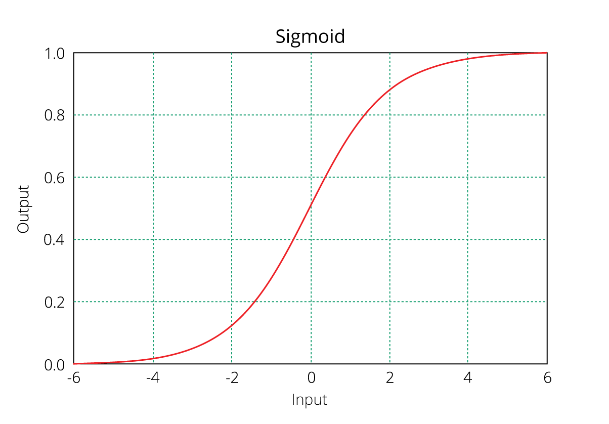
As you might recognize, the right side of the (immediate) equation above depicts the linear combination of independent variables. The left side is known as the log - odds or odds ratio or logit function and is the link function for Logistic Regression. This link function follows a sigmoid (shown below) function which limits its range of probabilities between 0 and 1.

SigmoidPlot logistic function

Until here, I hope you've understood how we derive the equation of Logistic Regression. But how is it interpreted?

We can interpret the above equation as, a unit increase in variable x results in multiplying the odds ratio by ? to power ?. In other words, the regression coefficients explain the change in log(odds) in the response for a unit change in predictor. However, since the relationship between p(X) and X is not straight line, a unit change in input feature doesn't really affect the model output directly but it affects the odds ratio.

This is contradictory to Linear Regression where, regardless of the value of input feature, the regression coefficient always represents a fixed increase/decrease in the model output per unit increase in the input feature.

In Multiple Regression, we use the Ordinary Least Square (OLS) method to determine the best coefficients to attain good model fit. In Logistic Regression, we use maximum likelihood method to determine the best coefficients and eventually a good model fit.

Maximum likelihood works like this: It tries to find the value of coefficients (?o,?1) such that the predicted probabilities are as close to the observed probabilities as possible. In other words, for a binary classification (1/0), maximum likelihood will try to find values of ?o and ?1 such that the resultant probabilities are closest to either 1 or 0. The likelihood function is written as

How can you evaluate Logistic Regression model fit and accuracy ?

In Linear Regression, we check adjusted R², F Statistics, MAE, and RMSE to evaluate model fit and accuracy. But, Logistic Regression employs all different sets of metrics. Here, we deal with probabilities and categorical values. Following are the evaluation metrics used for Logistic Regression:

1. Akaike Information Criteria (AIC)

You can look at AIC as counterpart of adjusted r square in multiple regression. It's an important indicator of model fit. It follows the rule: Smaller the better. AIC penalizes increasing number of coefficients in the model. In other words, adding more variables to the model wouldn't let AIC increase. It helps to avoid overfitting.

Looking at the AIC metric of one model wouldn't really help. It is more useful in comparing models (model selection). So, build 2 or 3 Logistic Regression models and compare their AIC. The model with the lowest AIC will be relatively better.

2. Null Deviance and Residual Deviance

Deviance of an observation is computed as -2 times log likelihood of that observation. The importance of deviance can be further understood using its types: Null and Residual Deviance. Null deviance is calculated from the model with no features, i.e.,only intercept. The null model predicts class via a constant probability.

Residual deviance is calculated from the model having all the features.On comarison with Linear Regression, think of residual deviance as residual sum of square (RSS) and null deviance as total sum of squares (TSS). The larger the difference between null and residual deviance, better the model.

Also, you can use these metrics to compared multiple models: whichever model has a lower null deviance, means that the model explains deviance pretty well, and is a better model. Also, lower the residual deviance, better the model. Practically, AIC is always given preference above deviance to evaluate model fit.

3. Confusion Matrix

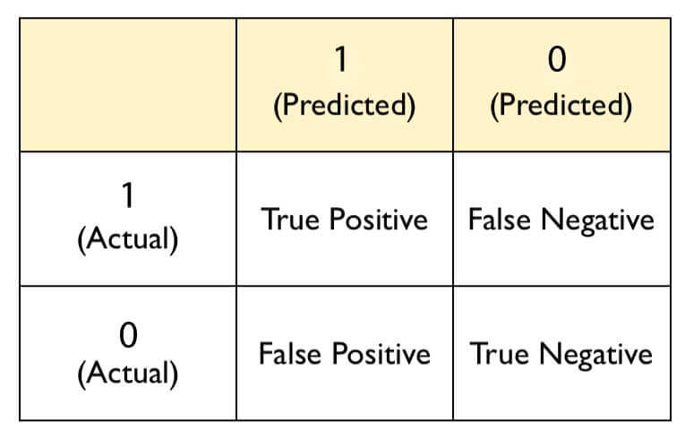
Confusion matrix is the most crucial metric commonly used to evaluate classification models. It's quite confusing but make sure you understand it by heart. If you still don't understand anything, ask me in comments. The skeleton of a confusion matrix looks like this:

confusion matrix logistic regression

As you can see, the confusion matrix avoids "confusion" by measuring the actual and predicted values in a tabular format. In table above, Positive class = 1 and Negative class = 0. Following are the metrics we can derive from a confusion matrix:

Accuracy - It determines the overall predicted accuracy of the model. It is calculated as Accuracy = (True Positives + True Negatives)/(True Positives + True Negatives + False Positives + False Negatives)

True Positive Rate (TPR) - It indicates how many positive values, out of all the positive values, have been correctly predicted. The formula to calculate the true positive rate is (TP/TP + FN). Also, TPR = 1 - False Negative Rate. It is also known as Sensitivity or Recall.

False Positive Rate (FPR) - It indicates how many negative values, out of all the negative values, have been incorrectly predicted. The formula to calculate the false positive rate is (FP/FP + TN). Also, FPR = 1 - True Negative Rate.

True Negative Rate (TNR) - It indicates how many negative values, out of all the negative values, have been correctly predicted. The formula to calculate the true negative rate is (TN/TN + FP). It is also known as Specificity.

False Negative Rate (FNR) - It indicates how many positive values, out of all the positive values, have been incorrectly predicted. The formula to calculate false negative rate is (FN/FN + TP).

Precision: It indicates how many values, out of all the predicted positive values, are actually positive. It is formulated as:(TP / TP + FP).

F Score: F score is the harmonic mean of precision and recall. It lies between 0 and 1. Higher the value, better the model. It is formulated as 2((precision*recall) / (precision+recall)).

Exclusive SQL Tutorial on Data Analysis in R

Introduction

Many people are pursuing data science as a career (to become a data scientist) choice these days. With the recent data deluge, companies are voraciously headhunting people who can handle, understand, analyze, and model data.

Be it college graduates or experienced professionals, everyone is busy searching for the best courses or training material to become a data scientist. Some of them even manage to learn Python or R, but still can't land their first analytics job!

What most people fail to understand is that the data science/analytics industry isn't just limited to using Python or R. There are several other coding languages which companies use to run their businesses.

Among all, the most important and widely used language is SQL (Structured Query Language). You must learn it.

I've realized that, as a newbie, learning SQL is somewhat difficult at home. After all, setting up a server enabled database engine isn't everybody's cup of tea. Isn't it? Don't you worry.

In this article, we'll learn all about SQL and how to write its queries.

Note: This article is meant to help R users who wants to learn SQL from scratch. Even if you are new to R, you can still check out this tutorial as the ultimate motive is to learn SQL here.

Table of Contents

  1. Why learn SQL ?
  2. What is SQL?
  3. Getting Started with SQL
    • Data Selection
    • Data Manipulation
    • Strings & Dates
  4. Practising SQL in R
Machine learning challenge, ML challenge

Why learn SQL ?

Good question! When I started learning SQL, I asked this question too. Though, I had no one to answer me. So, I decided to find it out myself.

SQL is the de facto standard programming language used to handle relational databases.

Let's look at the dominance / popularity of SQL in worldwide analytics / data science industry. According to an online survey conducted by Oreilly Media in 2016, it was found that among all the programming languages, SQL was used by 70% of the respondents followed by R and Python. It was also discovered that people who know Excel (Spreadsheet) tend to get significant salary boost once they learn SQL.

Also, according to a survey done by datasciencecentral, it was inferred that R users tend to get a nice salary boost once they learn SQL. In a way, SQL as a language is meant to complement your current set of skills.

Since 1970, SQL has remained an integral part of popular databases such as Oracle, IBM DB2, Microsoft SQL Server, MySQL, etc. Not only learning SQL with R will increase your employability, but SQL itself can make way for you in database management roles.

What is SQL ?

SQL (Structured Query Language) is a special purpose programming language used to manage, extract, and aggregate data stored in large relational database management systems.

In simple words, think of a large machine (rectangular shape) consisting of many, many boxes (again rectangles). Each box comprises a table (dataset). This is a database. A database is an organized collection of data. Now, this database understands only one language, i.e, SQL. No English, Japanese, or Spanish. Just SQL. Therefore, SQL is a language which interacts with the databases to retrieve data.

Following are some important features of SQL:

  1. It allows us to create, update, retrieve, and delete data from the database.
  2. It works with popular database programs such as Oracle, DB2, SQL Server, etc.
  3. As the databases store humongous amounts of data, SQL is widely known for it speed and efficiency.
  4. It is very simple and easy to learn.
  5. It is enabled with inbuilt string and date functions to execute data-time conversions.

Currently, businesses worldwide use both open source and proprietary relational database management systems (RDBMS) built around SQL.

Getting Started with SQL

Let's try to understand SQL commands now. Most of these commands are extremely easy to pick up as they are simple "English words." But make sure you get a proper understanding of their meanings and usage in SQL context. For your ease of understanding, I've categorized the SQL commands in three sections:

  1. Data Selection - These are SQL's indigenous commands used to retrieve tables from databases supported by logical statements.
  2. Data Manipulation - These commands would allow you to join and generate insights from data.
  3. Strings and Dates - These special commands would allow you to work diligently with dates and string variables.

Before we start, you must know that SQL functions recognize majorly four data types. These are:

  1. Integers - This datatype is assigned to variables storing whole numbers, no decimals. For example, 123,324,90,10,1, etc.
  2. Boolean - This datatype is assigned to variables storing TRUE or FALSE data.
  3. Numeric - This datatype is assigned to variables storing decimal numbers. Internally, it is stored as a double precision. It can store up to 15 -17 significant digits.
  4. Date/Time - This datatype is assigned to variables storing data-time information. Internally, it is stored as a time stamp.

That's all! If SQL finds a variable whose type is anything other than these four, it will throw read errors. For example, if a variable has numbers with a comma (like 432,), you'll get errors. SQL as a language is very particular about the sequence of commands given. If the sequence is not followed, it starts to throw errors. Don't worry I've defined the sequence below. Let's learn the commands. In the following section, we'll learn to use them with a data set.

Data Selection

  1. SELECT - It tells you which columns to select.
  2. FROM - It tells you columns to be selected should be from which table (dataset).
  3. LIMIT - By default, a command is executed on all rows in a table. This command limits the number of rows. Limiting the rows leads to faster execution of commands.
  4. WHERE - This command specifies a filter condition; i.e., the data retrieval has to be done based on some variable filtering.
  5. Comparison Operators - Everyone knows these operators as (=, !=, <, >, <=, >=). They are used in conjunction with the WHERE command.
  6. Logical Operators - The famous logical operators (AND, OR, NOT) are also used to specify multiple filtering conditions. Other operators include:
    • LIKE - It is used to extract similar values and not exact values.
    • IN - It is used to specify the list of values to extract or leave out from a variable.
    • BETWEEN - It activates a condition based on variable(s) in the table.
    • IS NULL - It allows you to extract data without missing values from the specified column.
  7. ORDER BY - It is used to order a variable in descending or ascending order.

Data Manipulation

  1. Aggregate Functions - These functions are helpful in generating quick insights from data sets.
    • COUNT - It counts the number of observations.
    • SUM - It calculates the sum of observations.
    • MIN/MAX - It calculates the min/max and the range of a numerical distribution.
    • AVG - It calculates the average (mean).
  2. GROUP BY - For categorical variables, it calculates the above stats based on their unique levels.
  3. HAVING - Mostly used for strings to specify a particular string or combination while retrieving data.
  4. DISTINCT - It returns the unique number of observations.
  5. CASE - It is used to create rules using if/else conditions.
  6. JOINS - Used to merge individual tables. It can implement:
    • INNER JOIN - Returns the common rows from A and B based on joining criteria.
    • OUTER JOIN - Returns the rows not common to A and B.
    • LEFT JOIN - Returns the rows in A but not in B.
    • RIGHT JOIN - Returns the rows in B but not in A.
    • FULL OUTER JOIN - Returns all rows from both tables, often with NULLs.
  7. ON - Used to specify a column for filtering while joining tables.
  8. UNION - Similar to rbind() in R. Combines two tables with identical variable names.

You can write complex join commands using comparison operators, WHERE, or ON to specify conditions.

sql joins data analysis data science

Strings and Dates

  1. NOW - Returns current time.
  2. LEFT - Returns a specified number of characters from the left in a string.
  3. RIGHT - Returns a specified number of characters from the right in a string.
  4. LENGTH - Returns the length of the string.
  5. TRIM - Removes characters from the beginning and end of the string.
  6. SUBSTR - Extracts part of a string with specified start and end positions.
  7. CONCAT - Combines strings.
  8. UPPER - Converts a string to uppercase.
  9. LOWER - Converts a string to lowercase.
  10. EXTRACT - Extracts date components such as day, month, year, etc.
  11. DATE_TRUNC - Rounds dates to the nearest unit of measurement.
  12. COALESCE - Imputes missing values.

These commands are not case sensitive, but consistency is important. SQL commands follow this standard sequence:

  1. SELECT
  2. FROM
  3. WHERE
  4. GROUP BY
  5. HAVING
  6. ORDER BY
  7. LIMIT

Practising SQL in R

For writing SQL queries, we'll use the sqldf package. It activates SQL in R using SQLite (default) and can be faster than base R for some manipulations. It also supports H2 Java database, PostgreSQL, and MySQL.

You can easily connect database servers using this package and query data. For more details, check the GitHub repo by its author.

When using SQL in R, think of R as the database machine. Load datasets using read.csv or read.csv.sql and start querying. Ready? Let’s begin! Code every line as you scroll. Practice builds confidence.

We'll use the babynames dataset. Install and load it with:

> install.packages("babynames")
> library(babynames)
> str(babynames)

This dataset contains 1.8 million observations and 5 variables. The prop variable is the proportion of a name given in a year. Now, load the sqldf package:

> install.packages("sqldf")
> library(sqldf)

Let’s check the number of rows in this data.

> sqldf("select count(*) from mydata")
#1825433

Ignore the warnings here. Next, let's look at the data — the first 10 rows:

> sqldf("select * from mydata limit 10")

* selects all columns. To select specific variables:

> sqldf("select year, sex, name from mydata limit 10")

To rename a column in the output using AS:

> sqldf("select year, sex as 'Gender' from mydata limit 10")

Filtering data with WHERE and logical conditions:

> sqldf("select year, name, sex as 'Gender' from mydata where sex == 'F' limit 20")
> sqldf("select * from mydata where prop > 0.05 limit 20")
> sqldf("select * from mydata where sex != 'F'")
> sqldf("select year, name, 4 * prop as 'final_prop' from mydata where prop <= 0.40 limit 10")

Ordering data:

> sqldf("select * from mydata order by year desc limit 20")
> sqldf("select * from mydata order by year desc, n desc limit 20")
> sqldf("select * from mydata order by name limit 20")

Filtering with string patterns:

> sqldf("select * from mydata where name like 'Ben%'")
> sqldf("select * from mydata where name like '%man' limit 30")
> sqldf("select * from mydata where name like '%man%'")
> sqldf("select * from mydata where name in ('Coleman','Benjamin','Bennie')")
> sqldf("select * from mydata where year between 2000 and 2014")

Multiple filters with logical operators:

> sqldf("select * from mydata where year >= 1980 and prop < 0.5")
> sqldf("select * from mydata where year >= 1980 and prop < 0.5 order by prop desc")
> sqldf("select * from mydata where name != '%man%' or year > 2000")
> sqldf("select * from mydata where prop > 0.07 and year not between 2000 and 2014")
> sqldf("select * from mydata where n > 10000 order by name desc")

Basic aggregation:

> sqldf("select sum(n) as 'Total_Count' from mydata")
> sqldf("select min(n), max(n) from mydata")
> sqldf("select year, avg(n) as 'Average' from mydata group by year order by Average desc")
> sqldf("select year, count(*) as count from mydata group by year limit 100")
> sqldf("select year, n, count(*) as 'my_count' from mydata where n > 10000 group by year order by my_count desc limit 100")

Using HAVING instead of WHERE for aggregations:

> sqldf("select year, name, sum(n) as 'my_sum' from mydata group by year having my_sum > 10000 order by my_sum desc limit 100")

Counting distinct names:

> sqldf("select count(distinct name) as 'count_names' from mydata")

Creating new columns using CASE (if/else logic):

> sqldf("select year, n, case when year = '2014' then 'Young' else 'Old' end as 'young_or_old' from mydata limit 10")
> sqldf("select *, case when name != '%man%' then 'Not_a_man' when name = 'Ban%' then 'Born_with_Ban' else 'Un_Ban_Man' end as 'Name_Fun' from mydata")

Joining data sets using a key:

> crash <- read.csv.sql("crashes.csv", sql = "select * from file")
> roads <- read.csv.sql("roads.csv", sql = "select * from file")
> sqldf("select * from crash join roads on crash.Road = roads.Road")
> sqldf("select crash.Year, crash.Volume, roads.* from crash left join roads on crash.Road = roads.Road")

Joining with aggregation and multiple keys:

> sqldf("select crash.Year, crash.Volume, roads.* from crash left join roads on crash.Road = roads.Road order by 1")
> sqldf("select crash.Year, crash.Volume, roads.* from crash left join roads on crash.Road = roads.Road where roads.Road != 'US-36' order by 1")
> sqldf("select Road, avg(roads.Length) as 'Avg_Length', avg(N_Crashes) as 'Avg_Crash' from roads join crash using (Road) group by Road")
> roads$Year <- crash$Year[1:5]
> sqldf("select crash.Year, crash.Volume, roads.* from crash left join roads on crash.Road = roads.Road and crash.Year = roads.Year order by 1")

String operations in sqldf with RSQLite extension:

> library(RSQLite)
> help("initExtension")

> sqldf("select name, leftstr(name, 3) as 'First_3' from mydata order by First_3 desc limit 100")
> sqldf("select name, reverse(name) as 'Rev_Name' from mydata limit 100")
> sqldf("select name, rightstr(name, 3) as 'Back_3' from mydata order by First_3 desc limit 100")

Summary

The aim of this article was to help you get started writing queries in SQL using a blend of practical and theoretical explanations. Beyond these queries, SQL also allows you to write subqueries aka nested queries to execute multiple commands in one go. We shall learn about those in future tutorials.

As I said above, learning SQL will not only give you a fatter paycheck but also allow you to seek job profiles other than that of a data scientist. As I always say, SQL is easy to learn but difficult to master. Do practice enough.

In this article, we learned the basics of SQL. We learned about data selection, aggregation, and string manipulation commands in SQL. In addition, we also looked at the industry trend of SQL language to infer if that's the programming language you will promise to learn in your new year resolution. So, will you?

If you get stuck with any query written above, do drop in your suggestions, questions, and feedback in comments below!

Beginners Tutorial on XGBoost and Parameter Tuning in R

Introduction

Last week, we learned about Random Forest Algorithm. Now we know it helps us reduce a model's variance by building models on resampled data and thereby increases its generalization capability. Good!

Now, you might be wondering, what to do next for increasing a model's prediction accuracy ? After all, an ideal model is one which is good at both generalization and prediction accuracy. This brings us to Boosting Algorithms.

Developed in 1989, the family of boosting algorithms has been improved over the years. In this article, we'll learn about XGBoost algorithm.

XGBoost is the most popular machine learning algorithm these days. Regardless of the data type (regression or classification), it is well known to provide better solutions than other ML algorithms. In fact, since its inception (early 2014), it has become the "true love" of kaggle users to deal with structured data. So, if you are planning to compete on Kaggle, xgboost is one algorithm you need to master.

In this article, you'll learn about core concepts of the XGBoost algorithm. In addition, we'll look into its practical side, i.e., improving the xgboost model using parameter tuning in R.

On 5th March 2017: How to win Machine Learning Competitions ?

Table of Contents

  1. What is XGBoost? Why is it so good?
  2. How does XGBoost work?
  3. Understanding XGBoost Tuning Parameters
  4. Practical - Tuning XGBoost using R

Machine learning challenge, ML challenge

What is XGBoost ? Why is it so good ?

XGBoost (Extreme Gradient Boosting) is an optimized distributed gradient boosting library. Yes, it uses gradient boosting (GBM) framework at core. Yet, does better than GBM framework alone. XGBoost was created by Tianqi Chen, PhD Student, University of Washington. It is used for supervised ML problems. Let's look at what makes it so good:

  1. Parallel Computing: It is enabled with parallel processing (using OpenMP); i.e., when you run xgboost, by default, it would use all the cores of your laptop/machine.
  2. Regularization: I believe this is the biggest advantage of xgboost. GBM has no provision for regularization. Regularization is a technique used to avoid overfitting in linear and tree-based models.
  3. Enabled Cross Validation: In R, we usually use external packages such as caret and mlr to obtain CV results. But, xgboost is enabled with internal CV function (we'll see below).
  4. Missing Values: XGBoost is designed to handle missing values internally. The missing values are treated in such a manner that if there exists any trend in missing values, it is captured by the model.
  5. Flexibility: In addition to regression, classification, and ranking problems, it supports user-defined objective functions also. An objective function is used to measure the performance of the model given a certain set of parameters. Furthermore, it supports user defined evaluation metrics as well.
  6. Availability: Currently, it is available for programming languages such as R, Python, Java, Julia, and Scala.
  7. Save and Reload: XGBoost gives us a feature to save our data matrix and model and reload it later. Suppose, we have a large data set, we can simply save the model and use it in future instead of wasting time redoing the computation.
  8. Tree Pruning: Unlike GBM, where tree pruning stops once a negative loss is encountered, XGBoost grows the tree upto max_depth and then prune backward until the improvement in loss function is below a threshold.

I'm sure now you are excited to master this algorithm. But remember, with great power comes great difficulties too. You might learn to use this algorithm in a few minutes, but optimizing it is a challenge. Don't worry, we shall look into it in following sections.

How does XGBoost work ?

XGBoost belongs to a family of boosting algorithms that convert weak learners into strong learners. A weak learner is one which is slightly better than random guessing. Let's understand boosting first (in general).

Boosting is a sequential process; i.e., trees are grown using the information from a previously grown tree one after the other. This process slowly learns from data and tries to improve its prediction in subsequent iterations. Let's look at a classic classification example:
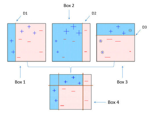
explain boosting

Four classifiers (in 4 boxes), shown above, are trying hard to classify + and - classes as homogeneously as possible. Let's understand this picture well.

  1. Box 1: The first classifier creates a vertical line (split) at D1. It says anything to the left of D1 is + and anything to the right of D1 is -. However, this classifier misclassifies three + points.
  2. Box 2: The next classifier says don't worry I will correct your mistakes. Therefore, it gives more weight to the three + misclassified points (see bigger size of +) and creates a vertical line at D2. Again it says, anything to right of D2 is - and left is +. Still, it makes mistakes by incorrectly classifying three - points.
  3. Box 3: The next classifier continues to bestow support. Again, it gives more weight to the three - misclassified points and creates a horizontal line at D3. Still, this classifier fails to classify the points (in circle) correctly.
  4. Remember that each of these classifiers has a misclassification error associated with them.
  5. Boxes 1,2, and 3 are weak classifiers. These classifiers will now be used to create a strong classifier Box 4.
  6. Box 4: It is a weighted combination of the weak classifiers. As you can see, it does good job at classifying all the points correctly.

That's the basic idea behind boosting algorithms. The very next model capitalizes on the misclassification/error of previous model and tries to reduce it. Now, let's come to XGBoost.

As we know, XGBoost can used to solve both regression and classification problems. It is enabled with separate methods to solve respective problems. Let's see:

Classification Problems: To solve such problems, it uses booster = gbtree parameter; i.e., a tree is grown one after other and attempts to reduce misclassification rate in subsequent iterations. In this, the next tree is built by giving a higher weight to misclassified points by the previous tree (as explained above).

Regression Problems: To solve such problems, we have two methods: booster = gbtree and booster = gblinear. You already know gbtree. In gblinear, it builds generalized linear model and optimizes it using regularization (L1,L2) and gradient descent. In this, the subsequent models are built on residuals (actual - predicted) generated by previous iterations. Are you wondering what is gradient descent? Understanding gradient descent requires math, however, let me try and explain it in simple words:

  • Gradient Descent: It is a method which comprises a vector of weights (or coefficients) where we calculate their partial derivative with respective to zero. The motive behind calculating their partial derivative is to find the local minima of the loss function (RSS), which is convex in nature. In simple words, gradient descent tries to optimize the loss function by tuning different values of coefficients to minimize the error.
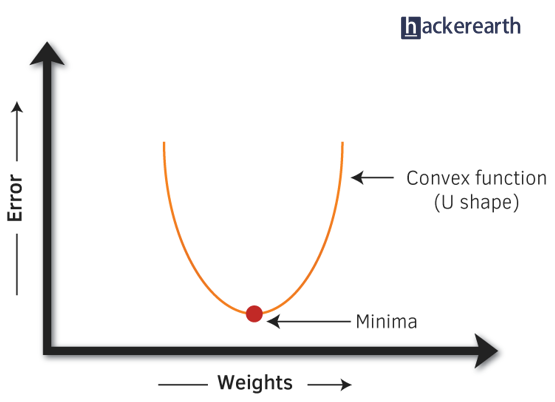
gradient descent convex function

Hopefully, up till now, you have developed a basic intuition around how boosting and xgboost works. Let's proceed to understand its parameters. After all, using xgboost without parameter tuning is like driving a car without changing its gears; you can never up your speed.

Note: In R, xgboost package uses a matrix of input data instead of a data frame.

Understanding XGBoost Tuning Parameters

Every parameter has a significant role to play in the model's performance. Before hypertuning, let's first understand about these parameters and their importance. In this article, I've only explained the most frequently used and tunable parameters. To look at all the parameters, you can refer to its official documentation.

XGBoost parameters can be divided into three categories (as suggested by its authors):
  • General Parameters: Controls the booster type in the model which eventually drives overall functioning
  • Booster Parameters: Controls the performance of the selected booster
  • Learning Task Parameters: Sets and evaluates the learning process of the booster from the given data

  1. General Parameters
    1. Booster[default=gbtree]
      • Sets the booster type (gbtree, gblinear or dart) to use. For classification problems, you can use gbtree, dart. For regression, you can use any.
    2. nthread[default=maximum cores available]
      • Activates parallel computation. Generally, people don't change it as using maximum cores leads to the fastest computation.
    3. silent[default=0]
      • If you set it to 1, your R console will get flooded with running messages. Better not to change it.

  2. Booster Parameters
  3. As mentioned above, parameters for tree and linear boosters are different. Let's understand each one of them:

    Parameters for Tree Booster

    1. nrounds[default=100]
      • It controls the maximum number of iterations. For classification, it is similar to the number of trees to grow.
      • Should be tuned using CV
    2. eta[default=0.3][range: (0,1)]
      • It controls the learning rate, i.e., the rate at which our model learns patterns in data. After every round, it shrinks the feature weights to reach the best optimum.
      • Lower eta leads to slower computation. It must be supported by increase in nrounds.
      • Typically, it lies between 0.01 - 0.3
    3. gamma[default=0][range: (0,Inf)]
      • It controls regularization (or prevents overfitting). The optimal value of gamma depends on the data set and other parameter values.
      • Higher the value, higher the regularization. Regularization means penalizing large coefficients which don't improve the model's performance. default = 0 means no regularization.
      • Tune trick: Start with 0 and check CV error rate. If you see train error >>> test error, bring gamma into action. Higher the gamma, lower the difference in train and test CV. If you have no clue what value to use, use gamma=5 and see the performance. Remember that gamma brings improvement when you want to use shallow (low max_depth) trees.
    4. max_depth[default=6][range: (0,Inf)]
      • It controls the depth of the tree.
      • Larger the depth, more complex the model; higher chances of overfitting. There is no standard value for max_depth. Larger data sets require deep trees to learn the rules from data.
      • Should be tuned using CV
    5. min_child_weight[default=1][range:(0,Inf)]
      • In regression, it refers to the minimum number of instances required in a child node. In classification, if the leaf node has a minimum sum of instance weight (calculated by second order partial derivative) lower than min_child_weight, the tree splitting stops.
      • In simple words, it blocks the potential feature interactions to prevent overfitting. Should be tuned using CV.
    6. subsample[default=1][range: (0,1)]
      • It controls the number of samples (observations) supplied to a tree.
      • Typically, its values lie between (0.5-0.8)
    7. colsample_bytree[default=1][range: (0,1)]
      • It control the number of features (variables) supplied to a tree
      • Typically, its values lie between (0.5,0.9)
    8. lambda[default=0]
      • It controls L2 regularization (equivalent to Ridge regression) on weights. It is used to avoid overfitting.
    9. alpha[default=1]
      • It controls L1 regularization (equivalent to Lasso regression) on weights. In addition to shrinkage, enabling alpha also results in feature selection. Hence, it's more useful on high dimensional data sets.

    Parameters for Linear Booster

    Using linear booster has relatively lesser parameters to tune, hence it computes much faster than gbtree booster.
    1. nrounds[default=100]
      • It controls the maximum number of iterations (steps) required for gradient descent to converge.
      • Should be tuned using CV
    2. lambda[default=0]
      • It enables Ridge Regression. Same as above
    3. alpha[default=1]
      • It enables Lasso Regression. Same as above

  4. Learning Task Parameters
  5. These parameters specify methods for the loss function and model evaluation. In addition to the parameters listed below, you are free to use a customized objective / evaluation function.

    1. Objective[default=reg:linear]
      • reg:linear - for linear regression
      • binary:logistic - logistic regression for binary classification. It returns class probabilities
      • multi:softmax - multiclassification using softmax objective. It returns predicted class labels. It requires setting num_class parameter denoting number of unique prediction classes.
      • multi:softprob - multiclassification using softmax objective. It returns predicted class probabilities.
    2. eval_metric [no default, depends on objective selected]
      • These metrics are used to evaluate a model's accuracy on validation data. For regression, default metric is RMSE. For classification, default metric is error.
      • Available error functions are as follows:
        • mae - Mean Absolute Error (used in regression)
        • Logloss - Negative loglikelihood (used in classification)
        • AUC - Area under curve (used in classification)
        • RMSE - Root mean square error (used in regression)
        • error - Binary classification error rate [#wrong cases/#all cases]
        • mlogloss - multiclass logloss (used in classification)

We've looked at how xgboost works, the significance of each of its tuning parameter, and how it affects the model's performance. Let's bolster our newly acquired knowledge by solving a practical problem in R.

Practical - Tuning XGBoost in R

In this practical section, we'll learn to tune xgboost in two ways: using the xgboost package and MLR package. I don't see the xgboost R package having any inbuilt feature for doing grid/random search. To overcome this bottleneck, we'll use MLR to perform the extensive parametric search and try to obtain optimal accuracy.

I'll use the adult data set from my previous random forest tutorial. This data set poses a classification problem where our job is to predict if the given user will have a salary <=50K or >50K.

Using random forest, we achieved an accuracy of 85.8%. Theoretically, xgboost should be able to surpass random forest's accuracy. Let's see if we can do it. I'll follow the most common but effective steps in parameter tuning:

  1. First, you build the xgboost model using default parameters. You might be surprised to see that default parameters sometimes give impressive accuracy.
  2. If you get a depressing model accuracy, do this: fix eta = 0.1, leave the rest of the parameters at default value, using xgb.cv function get best n_rounds. Now, build a model with these parameters and check the accuracy.
  3. Otherwise, you can perform a grid search on rest of the parameters (max_depth, gamma, subsample, colsample_bytree etc) by fixing eta and nrounds. Note: If using gbtree, don't introduce gamma until you see a significant difference in your train and test error.
  4. Using the best parameters from grid search, tune the regularization parameters(alpha,lambda) if required.
  5. At last, increase/decrease eta and follow the procedure. But remember, excessively lower eta values would allow the model to learn deep interactions in the data and in this process, it might capture noise. So be careful!

This process might sound a bit complicated, but it's quite easy to code in R. Don't worry, I've demonstrated all the steps below. Let's get into actions now and quickly prepare our data for modeling (if you don't understand any line of code, ask me in comments):

# set working directory
path <- "~/December 2016/XGBoost_Tutorial"
setwd(path)

# load libraries
library(data.table)
library(mlr)

# set variable names
setcol <- c("age",
            "workclass",
            "fnlwgt",
            "education",
            "education-num",
            "marital-status",
            "occupation",
            "relationship",
            "race",
            "sex",
            "capital-gain",
            "capital-loss",
            "hours-per-week",
            "native-country",
            "target")

# load data
train <- read.table("adultdata.txt", header = FALSE, sep = ",",
                    col.names = setcol, na.strings = c(" ?"),
                    stringsAsFactors = FALSE)
test <- read.table("adulttest.txt", header = FALSE, sep = ",",
                   col.names = setcol, skip = 1,
                   na.strings = c(" ?"), stringsAsFactors = FALSE)

# convert data frame to data table
setDT(train)
setDT(test)

# check missing values
table(is.na(train))
sapply(train, function(x) sum(is.na(x)) / length(x)) * 100
table(is.na(test))
sapply(test, function(x) sum(is.na(x)) / length(x)) * 100

# quick data cleaning
# remove extra character from target variable
library(stringr)
test[, target := substr(target, start = 1, stop = nchar(target) - 1)]

# remove leading whitespaces
char_col <- colnames(train)[sapply(test, is.character)]
for (i in char_col) set(train, j = i, value = str_trim(train[[i]], side = "left"))
for (i in char_col) set(test, j = i, value = str_trim(test[[i]], side = "left"))

# set all missing value as "Missing"
train[is.na(train)] <- "Missing"
test[is.na(test)] <- "Missing"

Up to this point, we dealt with basic data cleaning and data inconsistencies. To use xgboost package, keep these things in mind:

  1. Convert the categorical variables into numeric using one hot encoding
  2. For classification, if the dependent variable belongs to class factor, convert it to numeric

R's base function model.matrix is quick enough to implement one hot encoding. In the code below, ~.+0 leads to encoding of all categorical variables without producing an intercept. Alternatively, you can use the dummies package to accomplish the same task. Since xgboost package accepts target variable separately, we'll do the encoding keeping this in mind:

# using one hot encoding
>labels <- train$target
>ts_label <- test$target
>new_tr <- model.matrix(~.+0, data = train[,-c("target"), with = FALSE])
>new_ts <- model.matrix(~.+0, data = test[,-c("target"), with = FALSE])

# convert factor to numeric
>labels <- as.numeric(labels) - 1
>ts_label <- as.numeric(ts_label) - 1

For xgboost, we'll use xgb.DMatrix to convert data table into a matrix (most recommended):

# preparing matrix
>dtrain <- xgb.DMatrix(data = new_tr, label = labels)
&t;dtest <- xgb.DMatrix(data = new_ts, label = ts_label)

As mentioned above, we'll first build our model using default parameters, keeping random forest's accuracy 85.8% in mind. I'll capture the default parameters from above (written against every parameter):

# default parameters
params <- list(
    booster = "gbtree",
    objective = "binary:logistic",
    eta = 0.3,
    gamma = 0,
    max_depth = 6,
    min_child_weight = 1,
    subsample = 1,
    colsample_bytree = 1
)

Using the inbuilt xgb.cv function, let's calculate the best nround for this model. In addition, this function also returns CV error, which is an estimate of test error.

xgbcv <- xgb.cv(
    params = params,
    data = dtrain,
    nrounds = 100,
    nfold = 5,
    showsd = TRUE,
    stratified = TRUE,
    print.every.n = 10,
    early.stop.round = 20,
    maximize = FALSE
)
# best iteration = 79

The model returned lowest error at the 79th (nround) iteration. Also, if you noticed the running messages in your console, you would have understood that train and test error are following each other. We'll use this insight in the following code. Now, we'll see our CV error:

min(xgbcv$test.error.mean)
# 0.1263

As compared to my previous random forest model, this CV accuracy (100-12.63)=87.37% looks better already. However, I believe cross-validation accuracy is usually more optimistic than true test accuracy. Let's calculate our test set accuracy and determine if this default model makes sense:

# first default - model training
xgb1 <- xgb.train(
    params = params,
    data = dtrain,
    nrounds = 79,
    watchlist = list(val = dtest, train = dtrain),
    print.every.n = 10,
    early.stop.round = 10,
    maximize = FALSE,
    eval_metric = "error"
)

# model prediction
xgbpred <- predict(xgb1, dtest)
xgbpred <- ifelse(xgbpred > 0.5, 1, 0)

The objective function binary:logistic returns output predictions rather than labels. To convert it, we need to manually use a cutoff value. As seen above, I've used 0.5 as my cutoff value for predictions. We can calculate our model's accuracy using confusionMatrix() function from caret package.

# confusion matrix
library(caret)
confusionMatrix(xgbpred, ts_label)
# Accuracy - 86.54%

# view variable importance plot
mat <- xgb.importance(feature_names = colnames(new_tr), model = xgb1)
xgb.plot.importance(importance_matrix = mat[1:20])  # first 20 variables

xgboost variable importance plot

As you can see, we've achieved better accuracy than a random forest model using default parameters in xgboost. Can we still improve it? Let's proceed to the random / grid search procedure and attempt to find better accuracy. From here on, we'll be using the MLR package for model building. A quick reminder, the MLR package creates its own frame of data, learner as shown below. Also, keep in mind that task functions in mlr doesn't accept character variables. Hence, we need to convert them to factors before creating task:

# convert characters to factors
fact_col <- colnames(train)[sapply(train, is.character)]
for (i in fact_col) set(train, j = i, value = factor(train[[i]]))
for (i in fact_col) set(test, j = i, value = factor(test[[i]]))

# create tasks
traintask <- makeClassifTask(data = train, target = "target")
testtask <- makeClassifTask(data = test, target = "target")

# do one hot encoding
traintask <- createDummyFeatures(obj = traintask, target = "target")
testtask <- createDummyFeatures(obj = testtask, target = "target")

Now, we'll set the learner and fix the number of rounds and eta as discussed above.


#create learner
# create learner
lrn <- makeLearner("classif.xgboost", predict.type = "response")
lrn$par.vals <- list(
    objective = "binary:logistic",
    eval_metric = "error",
    nrounds = 100L,
    eta = 0.1
)

# set parameter space
params <- makeParamSet(
    makeDiscreteParam("booster", values = c("gbtree", "gblinear")),
    makeIntegerParam("max_depth", lower = 3L, upper = 10L),
    makeNumericParam("min_child_weight", lower = 1L, upper = 10L),
    makeNumericParam("subsample", lower = 0.5, upper = 1),
    makeNumericParam("colsample_bytree", lower = 0.5, upper = 1)
)

# set resampling strategy
rdesc <- makeResampleDesc("CV", stratify = TRUE, iters = 5L)

With stratify=T, we'll ensure that distribution of target class is maintained in the resampled data sets. If you've noticed above, in the parameter set, I didn't consider gamma for tuning. Simply because during cross validation, we saw that train and test error are in sync with each other. Had either one of them been dragging or rushing, we could have brought this parameter into action.

Now, we'll set the search optimization strategy. Though, xgboost is fast, instead of grid search, we'll use random search to find the best parameters.