Krunal M Harne

Data is key for making important business decisions. Depending upon the domain and complexity of the business, there can be many different purposes that a regression model can solve. It could be to optimize a business goal or find patterns that cannot be observed easily in raw data.

Even if you have a fair understanding of maths and statistics, using simple analytics tools you can only make intuitive observations. When more data is involved, it becomes difficult to visualize a correlation between multiple variables. You have to then rely on regression models to find patterns, which you can’t find manually, in the data.

In this article, we will explore different components of a data model and learn how to design a logistic regression model.

Before we start design a regression model, it is important to decide the business goal that you want to achieve with the analysis. It mostly revolves around minimizing or maximizing a specific (output) variable, which will be our Dependent variable (DV).

You must also understand the different metrics that are available or (in some cases) metrics that can be controlled to optimize the output. These metrics are called predictors or independent variables (IDVs).

A generalized linear regression equation can be represented as follows:

Y = β₀ + β₁X₁ + β₂X₂ + ... + βₚXₚ

where Xᵢ are the IDVs, βᵢ are the coefficients of the IDVs and β₀ is intercept.

This equation can be represented as follows:

Yᵢⱼ = Σₐ₌₁ᵖ Xᵢₐ βₐⱼ + eᵢⱼ

Logistic regression can be considered as a special case of linear regression where the DV is categorical or continuous. The output of this function is mostly probabilistic and lies between 0 to 1. Therefore, the equation of logistic regression can be represented in the exponential form as follows:

Y = 1 / (1 + e⁻ᶠ⁽ˣ⁾)

which is equivalent to:

Y = 1 / (1 + e⁻(β₀ + β₁X₁ + β₂X₂ + ... + βₚXₚ))

As you can see, the coefficients represent the contribution of the IDV to the DV. If Xᵢ is positive, then the high positive value increases the output probability whereas the high negative value of βᵢ decreases the output.

Once we fix our IDVs and DV, it is important to identify the data that is available at the point of decisioning. A relevant subset of this data can be the input of our equation, which will help us calculate the DV.

Two important aspects of the data are:

• Timeline of the data
• Mining the data

For example, if the data captures visits on a website, which has undergone suitable changes after a specific date, you might want to skip the past data for better decisioning. It is also important to rule out any null values or outliers, as required.

This can be achieved with a simple piece of code in R, which will have the following method:

Uploading the data from the .csv file and storing it as training.data. We shall use a sample data from imdb, which is available on Kaggle.

> training.data <- read.csv('movie_data.csv',header=T,na.strings=c(""))
> sapply(training.data,function(x) sum(is.na(x)))
color      director_name      num_critic_for_reviews      duration       director_facebook_likes  
19         104                50                          15             104
> training.data$imdb_score[is.na(training.data$imdb_score)] <- mean(training.data$imdb_score, na.rm=T)

You can also think of additional variables that can have a significant contribution to the DV of the model. Some variables may have a lesser contribution towards the final output. If the variables that you are thinking of are not readily available, then you can create them from the existing database.

When we are dealing with the non real-time data that we capture, we should be clear about how fast this data is captured so that it can provide a better understanding of the IDVs.

Building the model requires the following:

• Identifying the training data on which you can train your model
• Programming the model in any programming language, such as R, Python etc.

Once the model is created, you must validate the model and its efficiency on the existing data, which is of course different from the training data. To put it simply, it is estimating how your model will perform.

One efficient way of splitting the training and modelling data are the timelines. Assume that you have data from January to December, 2015. You can train the model on data from January to October, 2015. You can then use this model to determine the output on the data from November and December. Though you already know the output for November and December, you will still run the model to validate it.

You can arrange the data in chronological order and classify it as training and test data from the following array:

> train <- data[1:X,] 
> test <- data[X:last_value,]

Fitting the model includes obtaining coefficients of each of the predictors, z-value, and P-value etc. It estimates how close the estimated values of the IDVs in the equation are when compared to the original values.

We use the glm() function in R to fit the model. Here's how you can use it. The 'family' parameter that is used here is 'binomial'. You can also use 'poisson' depending upon the nature of the DV.

> reg_model <- glm(Y ~., family=binomial(link='logit'), data=train)
> summary(reg_model)
> glm(formula = Y ~ ., family = binomial(link = "logit"), data = train)

Let's use the following dataset which has 3 variables:

> trees
   Girth Height Volume
1    8.3     70   10.3
2    8.6     65   10.3
3    8.8     63   10.2
4   10.5     72   16.4
...

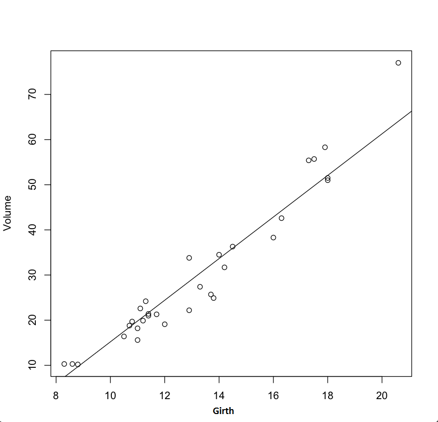
Fitting the model using the glm() function:

> data(trees)
> plot(Girth~Volume, data=trees)
> abline(model)
> plot(Volume~Girth, data=trees)
> model <- glm2(vol ~ gir, family=poisson(link="identity"))
> abline(model)
> model

Call:  glm2(formula = vol ~ gir, family = poisson(link = "identity"))

Coefficients:
(Intercept)          gir  
    -30.874        4.608  

Degrees of Freedom: 30 Total (i.e. Null);  29 Residual
Null Deviance:     247.3 
Residual Deviance: 16.54 	AIC: Inf

In this article, we have covered the importance of identifying the business objectives that should be optimized and the IDVs that can help us achieve this optimization. You also learned the following:

• Some of the basic functions in R that can help us analyze the model
• The glm() function that is used to fit the model
• Finding the weights of the predictors with their standard deviation

In our next article, we will use larger data-sets and validate the model that we will build by using different parameters like the KS test.

In the previous article, we saw how dplyr and tidyr packages in R can be used to visualize and plot data to gain a better understanding of the underlying properties. Now let’s explore the data visualization techniques in Python and see how similar tasks can be performed.

Pandas:

Pandas is a Python package aimed toward creating a platform to carry out practical data analysis and manipulation tasks. It has data structures that are equivalent to dataframe in R, and it can handle multiple types of data like SQL or Excel data, information present in the form of matrices, time series data, and labeled/unlabeled data. Here’s a preview of the tasks that can be carried out using Pandas:

1. groupby(..) function that is used to aggregate data through split-apply-combine operations
2. Merging, joining, slicing, reshaping and subsetting of data
3. Flexibility to change the dimension of data: addition and removal of columns
4. Handling of missing data similar to libraries in R

You can import Pandas just like you would import any other library in Python.

@ import pandas as pd

First step of dealing with Pandas involves reading data from a csv file.

@ data = pd.read_csv(file_path, header)

File_path: the location of the csv file to be read

Header: Can be None if you want the column heading to be Null. If column names are needed, then pass them as a list to the header argument.

After reading the data, placing it into a dataframe gives us the flexibility to perform various operations on it. To convert data into dataframe format use:

@ data_df = pd.DataFrame(data, column_list)

We are going to use the following dataframe in our later examples:

>>> marks_df

      names   marks

0     Ross      90
1     Joey      72
2     Monica    81
3     Phoebe    80
4     Chandler  45
5     Rachel    78

It is always important to have an estimate about the extreme values of the data. It is also convenient to have the data in a sorted format. To accomplish this, data can be sorted based on a column value in the dataframe using the sorting function:

@ df_sort = dataframe.sort_values(column, ascending)

column : column object of the dataframe

ascending: default value is True. If set to False, the data is sorted in descending order.

>>> list_sort = marks_df.sort_values(['marks'])
>>> list_sort

      names    marks
4    Chandler   45
1    Joey       72
5    Rachel     78
3    Phoebe     80
2    Monica     81
0    Ross       90

To get the entity with the maximum value (which is the last value in the sorted dataframe), tail(n) function can be used. n is the number of values from the last elements that need to be taken into consideration:

@ df_sort.tail(1)
>>> list_sort.tail(1)

   names  marks
0  Ross     90

Similarly, head() collects values from the top:

>> list_sort.head(2)

      names  marks
4   Chandler  45
1   Joey      72

Both head and tail, by default, will display 5 values from the top and bottom, respectively.

To get the information about the dataframe, use info():

@ marks_df.info()

>>> marks_df.info()
<class 'pandas.core.frame.DataFrame'>
RangeIndex: 6 entries, 0 to 5

Data columns (total 2 columns):
names    6 non-null object
marks    6 non-null int64

dtypes: int64(1), object(1)
memory usage: 168.0+ bytes

In the examples that follow, we are going to use the following dataframe that contains the complete exam results of all the 6 students (there are 6 subjects):

>>> allmarks_df

When there are multiple entries for each object, the aggregate option comes into play. We use the groupby() function to accomplish it. To get the total marks for each student, we need to aggregate all the name objects using the sum function:

@ agg_object = dataframe.groupby(column_name, as_index)

column_name: takes the list of columns based on which grouping needs to be done.

as_index: default value is True and means that the columns mentioned in list will be considered as indices for the new dataframe formed. When set to False, numerical numbering starting from 0 is given as the index.

>>> marks_agg = allmarks_df.groupby('Name')
>>> total_df = marks_agg.sum()
>>> total_df

Name      Marks      
Ross       495
Chandler   404
Rachel     422
Monica     443
Joey       475
Phoebe     395


>>> total_df = allmarks_df.groupby('Name', as_index=False).sum()
>>> total_df

      Name     Marks
0     Ross      495
1     Chandler  404
2     Rachel    422
3     Monica    443
4     Joey      475
5     Phoebe    395

Data can also be plotted using Pandas, but it requires pyplot from matplotlib:

>>> import matplotlib.pyplot as plt
>>> total_df['Marks'].plot(title="Total marks of all students")
<matplotlib.axes.AxesSubplot object at 0x10cde0d10>
>>> plt.show()

>>> total_df['Marks'].plot.bar()
<matplotlib.axes.AxesSubplot object at 0x10c2d1e90>
>>> plt.show()

To get the frequencies of the values in a particular column, use value_counts():

@ dataframe[column_name].value_counts()
>>> allmarks_df['Name'].value_counts()

Chandler   6
Ross       6
Rachel     6
Phoebe     6
Monica     6
Joey       6

Name: Name, dtype: int64

To get the unique values in a column:

@ dataframe[column_name].unique()
>>> allmarks_df['Name'].unique()
array(['Ross', 'Joey', 'Monica', 'Phoebe ', 'Chandler', 'Rachel'], dtype=object)

Dataframes can be accessed using the index too. ix() function is used to extract data using the index in numerical values:

@ dataframe.ix(index_range, columns_range)
>>> allmarks_df.ix[0:6,:]

      Name   Marks
0     Ross     77
1     Joey     73
2     Monica   80
3     Phoebe   58
4     Chandler 54
5     Rachel   51
6     Ross     98

>>> allmarks_df.ix[0:6,0]

0    Ross
1    Joey
2    Monica
3    Phoebe
4    Chandler
5    Rachel
6    Ross

Name: Name, dtype: object

>>> allmarks_df.ix[0:6,0:1]

       Name
0      Ross
1      Joey
2      Monica
3      Phoebe
4      Chandler
5      Rachel
6      Ross

Adding a column to data is quite easy in case of dataframe in Pandas:

@ dataframe[new_column] = value
>>> total_df['Pass'] = [total_df['Marks'][i] >= 420 for i in range(6)]
>>> total_df

Name      Marks   Pass             
Ross       495    True
Chandler   404    False
Rachel     422    True
Monica     443    True
Joey       475    True
Phoebe     395    False

loc() can be used to extract subset of a dataframe:

@ dataframe.loc[index / index_range]
>>> total_df.loc['Monica']

Marks     443
Pass     True

Name: Monica, dtype: object

>>> total_df.loc['Monica':'Phoebe ']

Name        Marks   Pass
Monica      443     True
Joey        475     True
Phoebe      395     False

iloc() is similar to loc() but here the index can be represented as numerals rather than as actual object names:

Subset of the dataframe can also be extracted by imposing a condition over the column values using logical operators:

>>> total_pass = total_df[total_df['Pass'] == True]
>>> total_pass

In the above example, all the rows with ‘Pass’ column value as True are separated out using the logical equality condition.

You can use the del function to delete a column.

@ del dataframe[column_name]
>>> del total_df['Pass']
>>> total_df

Data can be changed into different storage formats. stack() and unstack() functions are used for this. stack() is used to bring down the column names into index values and unstack() is used to revert the stacking action. Give it a try and see the output.

@ dataframe.stack()
>>> total_df.stack()
>>> total_df.unstack()

The rows and columns interchange positions after unstacking. We can revert this using the transpose function.

>>> total_df = total_df.T 
>>> total_df

Name     Ross  Chandler Rachel Monica Joey  Phoebe
Marks    495   404      422    443    475   395
Pass     True  False    True   True   True  False

>>> total_df = total_df.T
>>> total_df

Name     Marks   Pass
Ross      495    True
Chandler  404    False
Rachel    422    True
Monica    443    True
Joey      475    True
Phoebe    395    False

Subset of the dataframe can also be extracted by imposing a condition over the column values using logical operators:

>>> total_pass = total_df[total_df['Pass'] == True]
>>> total_pass

In the above example, all the rows with ‘Pass’ column value as True are separated out using the logical equality condition.

You can use the del function to delete a column.

@ del dataframe[column_name]
>>> del total_df['Pass']
>>> total_df

Data can be changed into different storage formats. stack() and unstack() functions are used for this. stack() is used to bring down the column names into index values and unstack() is used to revert the stacking action. Give it a try and see the output.

@ dataframe.stack()
>>> total_df.stack()
>>> total_df.unstack()

The rows and columns interchange positions after unstacking. We can revert this using the transpose function.

>>> total_df = total_df.T 
>>> total_df

Name     Ross  Chandler Rachel Monica Joey  Phoebe
Marks    495   404      422    443    475   395
Pass     True  False    True   True   True  False

>>> total_df = total_df.T
>>> total_df

Name     Marks   Pass
Ross      495    True
Chandler  404    False
Rachel    422    True
Monica    443    True
Joey      475    True
Phoebe    395    False

Subset of the dataframe can also be extracted by imposing a condition over the column values using logical operators:

>>> total_pass = total_df[total_df['Pass'] == True]
>>> total_pass

In the above example, all the rows with ‘Pass’ column value as True are separated out using the logical equality condition.

You can use the del function to delete a column.

@ del dataframe[column_name]
>>> del total_df['Pass']
>>> total_df

Data can be changed into different storage formats. stack() and unstack() functions are used for this. stack() is used to bring down the column names into index values and unstack() is used to revert the stacking action. Give it a try and see the output.

@ dataframe.stack()
>>> total_df.stack()
>>> total_df.unstack()

The rows and columns interchange positions after unstacking. We can revert this using the transpose function.

>>> total_df = total_df.T 
>>> total_df

Name     Ross  Chandler Rachel Monica Joey  Phoebe
Marks    495   404      422    443    475   395
Pass     True  False    True   True   True  False

>>> total_df = total_df.T
>>> total_df

Name     Marks   Pass
Ross      495    True
Chandler  404    False
Rachel    422    True
Monica    443    True
Joey      475    True
Phoebe    395    False

Mean and standard deviation for a particular value of the data can be calculated using standard functions. Mean: mean() and standard deviation: std()

@ dataframe[column_name].mean()
@ dataframe[column_name].std()

>>> total_df['Marks'].mean()
439.0

>>> total_df['Marks'].std()
39.744181964156716

>>> total_df['dis-Mean'] = total_df['Marks'] - total_df['Marks'].mean()
>>> total_df

      Name    Marks  dis-Mean
0     Ross      495      56.0
1     Chandler  404     -35.0
2     Rachel    422     -17.0
3     Monica    443       4.0
4     Joey      475      36.0
5     Phoebe    395     -44.0

The above example adds a column to the dataframe containing the deviation from the mean value of Marks.

Generating a time series data:

>>> time = pd.date_range('1/1/2012', periods=48, freq='MS')
>>> time

DatetimeIndex(['2012-01-01', '2012-02-01', '2012-03-01', '2012-04-01',
               '2012-05-01', '2012-06-01', '2012-07-01', '2012-08-01',
               '2012-09-01', '2012-10-01', '2012-11-01', '2012-12-01',
               '2013-01-01', '2013-02-01', '2013-03-01', '2013-04-01',
               '2013-05-01', '2013-06-01', '2013-07-01', '2013-08-01',
               '2013-09-01', '2013-10-01', '2013-11-01', '2013-12-01',
               '2014-01-01', '2014-02-01', '2014-03-01', '2014-04-01',
               '2014-05-01', '2014-06-01', '2014-07-01', '2014-08-01',
               '2014-09-01', '2014-10-01', '2014-11-01', '2014-12-01',
               '2015-01-01', '2015-02-01', '2015-03-01', '2015-04-01',
               '2015-05-01', '2015-06-01', '2015-07-01', '2015-08-01',
               '2015-09-01', '2015-10-01', '2015-11-01', '2015-12-01'],
              dtype='datetime64[ns]', freq='MS')

>>> stock = pd.DataFrame([np.random.randint(low=0, high=50) for i in range(48)], index=time, columns=['Value'])
>>> stock['dev'] = stock['Value'] - stock['Value'].mean()
>>> stock

             Value       dev
2012-01-01     37   10.104167
2012-02-01     48   21.104167
2012-03-01     41   14.104167
2012-04-01      5  -21.895833
2012-05-01     13  -13.895833
2012-06-01      7  -19.895833
2012-07-01     37   10.104167
2012-08-01     31    4.104167
2012-09-01     32    5.104167
2012-10-01     46   19.104167
2012-11-01     40   13.104167
2012-12-01     18   -8.895833
2013-01-01     38   11.104167
2013-02-01     23   -3.895833
2013-03-01     17   -9.895833
2013-04-01     21   -5.895833
2013-05-01     12  -14.895833
2013-06-01     40   13.104167
2013-07-01      9  -17.895833
2013-08-01     47   20.104167
2013-09-01     42   15.104167
2013-10-01      3  -23.895833
2013-11-01     24   -2.895833
2013-12-01     38   11.104167
2014-01-01     33    6.104167
2014-02-01     41   14.104167
2014-03-01     25   -1.895833
2014-04-01     11  -15.895833
2014-05-01     44   17.104167
2014-06-01     47   20.104167
2014-07-01      6  -20.895833
2014-08-01     49   22.104167
2014-09-01     11  -15.895833
2014-10-01     14  -12.895833
2014-11-01     23   -3.895833
2014-12-01     35    8.104167
2015-01-01     23   -3.895833
2015-02-01      1  -25.895833
2015-03-01     46   19.104167
2015-04-01     49   22.104167
2015-05-01     16  -10.895833
2015-06-01     25   -1.895833
2015-07-01     22   -4.895833
2015-08-01     36    9.104167
2015-09-01     30    3.104167
2015-10-01      3  -23.895833
2015-11-01     12  -14.895833
2015-12-01     20   -6.895833

Plotting the value of stock over 4 years using pyplot:

>>> stock['Value'].plot()
<matplotlib.axes.AxesSubplot object at 0x10a29bb10>
>>> plt.show()

>>> stock['dev'].plot.bar() 
<matplotlib.axes.AxesSubplot object at 0x10c3e09d0>
>>> plt.show()

There are more plotting tools like the seaborn library that can create more sophisticated plots. With these data visualization packages in R and Python, we are ready to advance to the core concepts of Machine Learning.

We have our Machine Learning practice section coming soon. Stay tuned.

A good understanding of data is one of the key essentials to designing effective Machine Learning (ML) algorithms. Realizing the structure and properties of the data that you are working with is crucial in devising new methods that can solve your problem. Visualizing data includes the following:

• Cleaning up the data
• Structuring and arranging it
• Plotting it to understand the granularity

R, one of the few widely-used programming languages for ML, has many data-visualization libraries.

In this article, we will explore two of the most commonly used packages in R for analyzing data—dplyr and tidyr.

Using dplyr and tidyr

dplyr and tidyr, created by Hadley Wickham and maintained by the RStudio team, offer a powerful set of tools for data manipulation. One of their best features is the pipeline operator %>%, which allows chaining multiple operations together in a clean and readable format.

tidyr Functions

gather()

Transforms wide-format data into long-format by collecting columns into key-value pairs.

gather(data, key, value, ..., na.rm = FALSE, convert = FALSE, factor_key = FALSE)
data %>% gather(key, value, ..., na.rm = FALSE, convert = FALSE, factor_key = FALSE)

spread()

Opposite of gather(); spreads key-value pairs into wide format.

spread(data, key, value, fill = NA, convert = FALSE, drop = TRUE, sep = NULL)

separate() & unite()

separate() splits a column into multiple columns based on a separator. unite() merges multiple columns into one.

dplyr Functions

select()

Choose specific columns based on name, pattern, or position.

filter(), slice(), distinct(), sample_n(), sample_frac()

Filter rows, remove duplicates, and take samples from the data.

group_by() & summarise()

group_by() creates groups, while summarise() computes summary statistics for each group.

summarise(df, avg = mean(column_name))

mutate()

Add or transform columns using expressions like:

mutate(new_col = col1 / col2)

Joins

Supports all major joins: left_join(), right_join(), inner_join(), full_join(), semi_join(), and anti_join().

arrange()

Sort data ascending or descending using desc().

Data Visualization with ggplot2

Bar Chart Example

ggplot(data = gather(stocks, stock, price, -time) %>%
       group_by(time) %>%
       summarise(avg = mean(price)),
       aes(x = time, y = avg, fill = time)) +
       geom_bar(stat = "identity")

Scatter Plot Example

qplot(time, avg,
      data = gather(stocks, stock, price, -time) %>%
             group_by(time) %>%
             summarise(avg = mean(price)),
      colour = 'red',
      main = "Avg change of stock price for each month",
      xlab = "month",
      ylab = "avg price")

Regression models help uncover hidden trends. Libraries like dplyr and tidyr don’t just clean your data—they boost your data intuition and enable better decisions.

In the next article, we'll explore more data-visualization libraries.

We live in an interesting era in the history of mankind. You will be surprised to know that Apollo 11, the computer that put Man on the Moon in 1969, whose assembly language code was recently published on Github, operated on 64KB memory whereas today’s kids have 64GB iPhones to click duckface selfies to upload on Instagram and play PokeMon Go, a viral game that marginally broke all time daily active users’ record in a week! Technically, 1 Million times more memory and 100 million times computational power at your disposal. After all, Moore’s law is nothing less than a super genius prediction.

Thought provoking extrapolation of the same Moore’s law, that says that the number of transistors in an integrated circuit and hence the computational power doubles itself every 2 years resulting into exponential technological growth, is applicable to the most evolving field of technology, Artificial Intelligence. For me, as the kid of Gen-Y, it is mind-blowing to think how the first movie ever was produced in the year my great grandfather was born, the first computer was built when my grandfather was still in his teens, the first Star Wars movie was released when my father learned fishing and how only last month, I blew my mind watching the first movie named Sunspring written by an AI program that christened itself as Benjamin. Not going to be long before I know, my kid wakes me up in the middle of the night someday and tells me, ‘Hey dad! One super intelligent robot called Trump has waged a war against humanity to destroy the entire human race.’ And WHAM! The most dreaded Apocalypse is a reality. Who knows?

If you are still optimistic and think that it is just a trippy thought experiment, here’s the generalized version of Moore’s law, depicted by Kurzweil as The Law of Accelerating Returns.

Kurzweil provides an interesting way of looking at the advancement of Artificial in terms of CPS achieved per $1000. The exponential nature of this curve can be visualized with respect to human intelligence and how quickly we are advancing towards the human level intelligence.

Not a long ago, we were struggling to artificially replicate the brain, read intelligence, of an insect and just so overwhelmingly, we are not too far from artificially achieving the intelligence of the most superior specie on the planet earth. What lies beyond that is a mystery for a layman but we indeed are living in the golden era of the exponential curve of technological progress. The singularity is near!

The journey so far hasn’t been easy. Ponder over this deep. Starting from the Big bang, to the birth of life on the earth, to development of human civilizations, to the million science experiments that went wrong along the progress including the first computer and the first lines of code, followed by a gazillion more, everything has contributed in making today’s Machine learn with humongous data to take intelligent decisions of its own, to probably build their own society tomorrow.

The Need of Artificial Intelligence

Have you ever been so lazy to be stalled on your bed with packets of tortilla chips and the latest episodes of Game of Thrones, that you just fantasized a remote control with multiple buttons to open the door or turn the fan on or do all that boring stuff? Oh wait, that still requires you to hold the remote and press the buttons, right? Gee, why don’t we have a robot that would just read our mind and do everything from household stuff to attending the unwanted guests without asking anything in return. Firstly, such robot will have to be super intelligent. Not only will it have to be efficient to perform routine tasks, but also understand your emotions viz-a-viz, mood swings and your behavioral pattern by observing you every minute and processing the data of your actions and emotions. Apart from the hard-coded seemingly basic set of functions, which in itself is a mammoth task, the machine will have to progressively learn by observations in order to perform as good as a smart human to serve you.

While a lot of this has been significantly achieved, it is still a very hard task for a machine to detect, segregate and arrange scented towels, hairdryers, Nutella box or contact lenses from a pile of junk than computing the complicated Euler product for a Riemann Zeta function. Machines can be entirely clueless and result into wrong outputs for what seems obvious that humans can solve in just a second’s glance.

You know how they say, “Don’t reinvent the wheel”, researchers have recently recreated a complex Quantum Physics experiment using AI just in an hour, that had won a Nobel prize in 2001 followed by years of determination and hard work by renowned Physicists like Einstein and Bose. We need AI to take care of trivial life problems so that we can invest our time and build a better AI to solve more important problems, like treating cancer or fighting against global warming. Fascinatingly enough, AI is actually everywhere; but more often than not we fail to see it. Because as John McCarthy, rightly says: “As soon as it works, no one calls it AI anymore.”

How AI is Everywhere Facilitated by Machine Learning

Right from a smartphone App that suggests you the nearby fast food outlet you might be interested in, to Facebook’s photo tagging Algorithm that detects your face with or without a beard, to Google’s self driving car, AI is everywhere and is deeply embedded in our lives without us realizing it. Our perceptions of AI are biased by Sci-Fi movies with evil machines trying to take over the galaxy. Intelligent machines designed to learn in order to become more intelligent by themselves to achieve Superintelligence is not hard to imagine. Technically, this would lie on the steepest slope of the exponential curve of intelligence versus time that we discussed before.

It is a beautiful realization that the roots of Artificial intelligence of a self driving car taking decisions that involve lives on the road lie within countless trivial and complicated Machine Learning algorithms that actually start with a few lines of code on your computer. My friend who had no background of computer science whatsoever before college, started learning programming in his sophomore year and took a long time before he could write fine algorithms in C++. He then started reading about Image processing, right from how a black and white image can be represented with a metric of numbers and went on writing a simple algorithm to detect a stable human hand. Soon with his growing interest, the human hand was replaced with colonoscopy images to robust deep learning algorithms that could detect cancer with image processing. His research paper got accepted in an international conference and has many other industrial applications.

Machine Learning and the Power of Big Data

With unmatched computational power machines can process and be trained to make decisions using big data and predictive modelling. Imagine a person having superpowers who can predict future of everything, the world would fall at their feet. In a more logical sense, if a machine can process humongous amount of historical and real time data with prediction models, and learns over time to get better and better, imagine, the power of big data is nothing less than magical.

Several industries vastly use Machine Learning to take data driven decisions and make life smarter with the power of data accumulated over the years. Healthcare has already been positively impacted with the tremendous amount of work in this field that has contributed in saving thousands of lives. From Governance to Economy to Healthcare, name a domain and you have smart multi-variable regression models backed by big data, performing predictive analysis. Super intelligent machines can now decide your fate to survive in a Multi-Billion dollar stock market. In a way, AI has started affecting our lives tangibly even without us realizing it, and if you look back, it really happened in the blink of an eye.

Whether we live to see the empire of Artificial Superintelligence that surpasses our brain and the human race ends up being the “biological boot loader for digital Superintelligence” OR we produce extraordinary artificial intelligence to look beyond galaxies and travel to future, only time will tell. But one thing is for sure, whatever happens, at the heart of it lie several complicated Algorithms that actually started with a few lines of code.